Sleep State Detection Method by Data-generated likelihood
Published
Yeonsook Kwak*
* Swiss Institute of Artificial Intelligence, Chaltenbodenstrasse 26, 8834 Schindellegi, Schwyz, Switzerland
Sleep research using accelerometers from wearable devices is less precise than existing polysomnography. By contrast, An ever-increasing number of studies use accelerometer data that offers continuous, longitudinal, and noninvasive measurements. In this paper, we discuss a generalized approach for detecting sleep states that are subject to finding asleep and awake points by using linear transformed summary metric ‘ENMO’ signal data from the accelerometer of a wrist-worn watch. In particular,We propose to present a generalized method from two perspectives. First by applying a preprocessing method in the irregular signal data to ensure consistent signal in some repetitive sleep period. The other suggests the generalised model structure by using distribution. In contrast to prior studies, which have predominantly concentrated on optimized concepts such as machine learning, deep learning, or other regression-based models, the primary objective of this model lies in maximizing the information value it extracts, that can be applied to short-term datasets throughout a minimum duration of one day.
1. Introduction
In sleep analysis, there are classical methods. One is sleep diaries which is similar to cohort analysis based on participants’ questions and answers. Normally the question is “when do you sleep or when do you wake up?”. It is dependent on participants’ reports. Therefore there are possibilities to be biased. The other is polysomnography which is usually used as the gold standard.
In comparison to polysomnography, renowned for its superior precision, research on sleep assessment using both accelerometers and photoplethysmography together is increasing. This surge in interest stems from the convenience offered by wearable devices, facilitating easy measurement. As a result of constraints arising from data limitations, this study extensively focuses on the detection of sleep states exclusively using accelerometer data, excluding photoplethysmography data.
Primarily, wearable sensors can offer continuous, longitudinal, non-invasive measurements, providing various insights into physical activity, sleep, and circadian rhythm changes. Therefore the conventional UK Biobank[4] approach was also used as a different type of cohort analysis where a sleep diary was not used.
This study aims to detect sleep states using accelerometer sensor data and sleep diaries (cohort analysis) as standard label data. Hence, this research focused on sleep state detection, not sleep stage discrimination.
When employing an accelerometer signal, it’s essential to evaluate its capacity to discern different types of acceleration. Consequently, direct discrimination between acceleration caused by gravity and other accelerations may not be straightforward. Instead, it measures the total acceleration vector acting on the device in three dimensions(x, y, and z axes). Figure 1 shows accelerometer x, y, and z signal data. In this graph, you can see from accelerometer data collected by a worn device shows how walking is measured differently between when arms are under movement or stationary during normal walking. In particular, changes in the x, y, and z device directions appear as changes in the average value, most clearly seen in the signal shown in green line.[6]
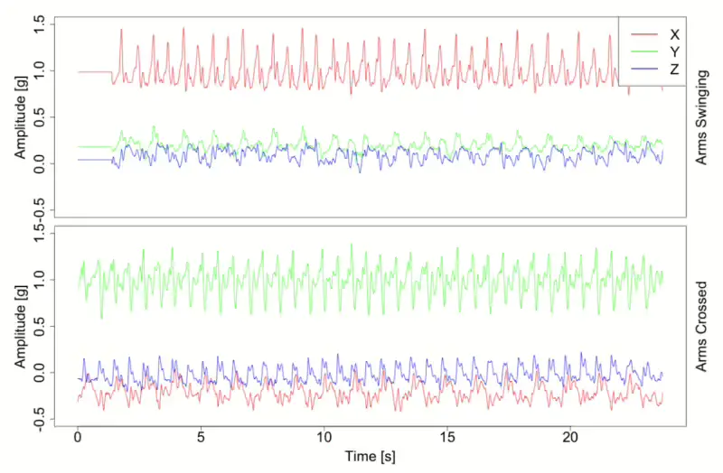
We can think that the x is forwarding movements from the ground, and the y-axis explains the changes in how much we shake our arms, and the z-axis represents the change in direction of jumping vertically from the ground. However, if the function of each axis changes, and the base axis of the sensor changes, movement is usually checked based on the value with the largest change in the overall value. Therefore, if we use raw tri-axial signals, base axis consideration may be important because values must be considered according to a certain position(Figure 1). However, using standardized summary measurement can alleviate and trivialise this reference axis point problem. Therefore we could handle the base direction problem even if we ignore the bias on the transformed variable. A variety of transformed variables like ENMO, VMC and AI, Angle-z[1, 11, 14] that are called summary measurements have been developed, which are all rotation invariant.
Although the perspectives are not completely the same, to isolate the effect of gravity from the total acceleration and to lessen the base direction problem, we are going to apply ENMO summary measurement.
Sundarajan et al.[5]proposed a random forest model for detecting sleep state with statistical measures. Random forest is an ensemble learning method that constructs multiple decision trees during the training process and the final output is the mode of the classes output by each individual decision trees. Here, reported Locomotor Inactivity During Sleep(LIDS) and Z-angle are the most important features for sleep-wake classification. Similarly, within the scope of this research, Random Forests were employed to ascertain the representativeness of the variable. Additionally, this study investigated the feature importance of mean variables at 1-minute intervals for both the z-angle and ENMO using a Random Forest for each tree.
Most of the analyses of the random forest tree’s feature importance revealed that the rolling mean associated with ENMO exhibited high significance, whereas variables like angle-z did not rank within the top 10. Notably, among the angle-z variables, angle-z10, representing the average sensor data value between 5 to 6 minutes following the event, emerged as the most pivotal, as depicted in the top graph (Figure 2).
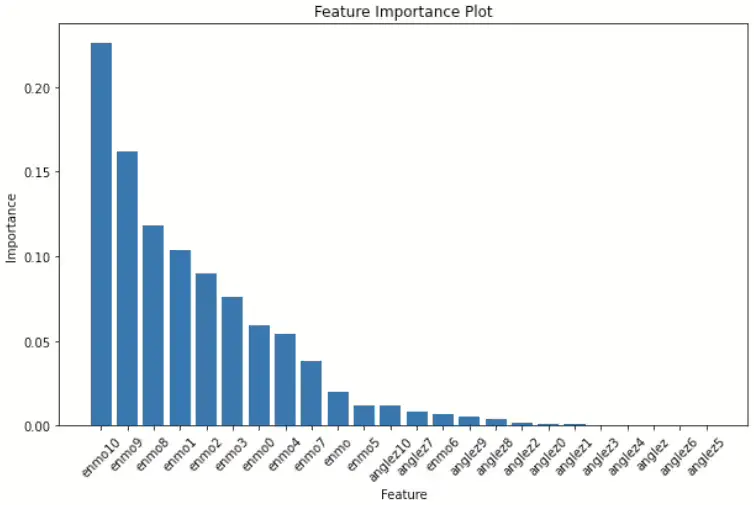
Consequently, it is apparent from this analysis that among the variables under consideration, the ENMO variable holds greater significance compared to others, suggesting it may serve as the primary determinant rather than utilizing both variables in tandem.
1.1. Related Work
In this section, we provide a brief outline of previous work done in sleep state detection and detailed research and related validation metric.
When examining the intricacy of the model, it becomes apparent that machine learning models such as random forest, and artificial neural network models like CNN and LSTM (as discussed by Sundararajan et al.[5] and and Palotti et al.[10]), exhibit significant complexity. Due to their prioritization of accuracy, these models often encounter discarded data points. Indeed, It is tricky to capture the nuanced difference between heading to bed and falling asleep (or, conversely, waking up and getting out of bed) with time interval statistics. This situation parallels an overemphasis on mitigating type 1 errors (i.e. concerns regarding false alarms) at the expense of neglecting type 2 errors (i.e. misidentification). Overly fixating on optimization may exacerbate imbalances, leading to the detection of only type 1 errors while overlooking type 2 errors.
Cole-Kripke et al.[3] and Oakley et al.[9] emphasize that their regression models exhibit lower complexity levels compared to existing machine learning or deep learning models, using aggregate called counts. Oakley et al. suggest threshold was selected using the training data to maximize the F1 score. Results of both optimized threshold and medium setting are reported for comparison. Oakley et al. entail a regression equation comprising activity scores and weights from the current time, previous time, and subsequent time.
Employing overlapping epochs lasting up to 10 seconds, this approach generates scores every minute. It applies a regression equation to training sample data and iteratively adjusts parameters to optimize the discrimination ratio between sleep and wake states.
As the regression model operates under the assumption of normality, both of the aforementioned regression models necessitated highly sophisticated optimization techniques as a means to address deviations from normality.
In general, when data with entirely distinct patterns is introduced from existing studies, there exists a considerable tendency that the models outlined in those studies will not align well. Moreover, numerous instances may arise where classification or detection fails to function adequately with short-term data. This phenomenon occurs due to the challenge of detecting subtle nuances between asleep and awake states, particularly when utilizing statistics such as 5-minute or 1-minute intervals, where the previous value often reflects a near-steady state, complicating the detection process.
The evaluation metrics[7] commonly utilized in existing sleep research include sensitivity (measuring agreement between actigraphy and PSG when both indicate sleep), specificity (measuring agreement between actigraphy and PSG when both indicate wakefulness), accuracy, wakefulness after sleep onset (WASO), and sleep efficiency (SE). However, in this study, a direct 1:1 comparison of data is not feasible, highlighting the limitations of solely focusing on accuracy. Therefore, referencing the approach proposed by Van Hee et al.[12], this study aims to incorporate the time difference between the labeled values and the predicted values as a comparative metric.
2. Data explanantion
Especially, Interpreting accelerometer data is an open and challenging problem due to the high heterogeneity of data, both within- and between-subjects. Although it would be better to consider user acceptance (i.e. demographic characteristics, patient type, disorders of maintaining sleep(DIMS), etc.), this study consists of data designed for children provided by Healthy Brain Network from https://healthybrainnetwork.org. The dataset utilized in this study comprised ENMO and angle-z variables, both converted using the GGIR package[8].
ENMO (Euclidean Norm Minus One (1g = 9.81ms-2)) :
(1)ENMO=max(0,x2+y2+z2–1)
Angle-z (the angle of the arm relative to the vertical axis of the body) :
(2)angleZ=tan−1(azax2+ay2)⋅180π
Figure 3 shows sampling 10ea ID density graph of ENMO and angle-z respectively. ENMO looks like a right-skewed shape and angle-z seems like a normal distribution shape. Bakrania et al.[2] proposed specific sedentary types that are difficult to distinguish when concerned with sensor position, depending on whether it is writ or hip. This data was collected from a wrist-worn device. Under normal circumstances, it may be deduced that a sensor worn at the hip could potentially provide greater accuracy in distinguishing activities upon awakening. This will be more pronounced when the value of the angle is related. However, we do have only wrist-worn collected data, given the robust representativeness of ENMO, it is considered sufficient to utilize only this variable in the subsequent methodology, as previously suggested with feature importance(Figure 2).
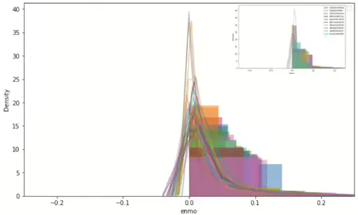
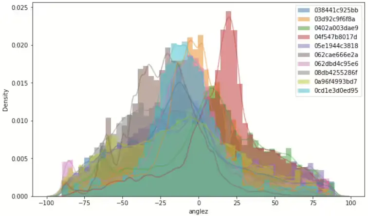
Figure 3. Left shows total ENMO signal density graph and top right of same frame shows 10ea sample ID’s density graph. And right shows 10ea sample ID’s density graph of angle-z
The ENMO signal to be used is from the data collected at 5-second intervals in conjunction with sleep diary label values for sleep state detection. The sleep diary label values are derived from subjective reports provided by participants. Here are the specific restrictions associated with these label values as documented in the sleep diary.
- A single sleep period must be at least 30 minutes in length.
- Sleep events do not need to overlap the day-line, and therefore there is no hard and fast rule defining how many may occur within a given period. However, no more than one window should be assigned per night. For example, it is valid for an individual to have a sleep window from 01h:00–06h:00 and 19h:00–23h:30 in the same calendar day, though assigned to consecutive nights.
- Assume that no one has certain robot-like movements such as unchanged steady state.
The total dataset comprises 124,822,080 individual data points for the signal and 14,508 data points for the labels. We utilized the entire dataset to analyze the characteristics of the distribution and signal processing. However, for later result verification, we only used a subset of the data. This approach allowed us to comprehensively explore the dataset’s properties while ensuring efficient processing and validation of results.
This study focuses on characteristics, considering the periodicity inherent in the data. Furthermore, while individuals may exhibit unique sleep patterns, there is a commonality in the repetition of sleeping and waking periods.
3. Methodology
In order to improve the problems of existing studies mentioned in section 1.1, We would like to propose a generalized methodology in Section 3.
Usually, a process called regularization will be performed to improve some of the problems similar to the above (i.e. overfitting). For example, Support vector machines(SVM) use hyperplane seperating the data points. The objective function for an SVM classifier is:
(3)minw,b,ξ||w||22+C∑i=1nξiwith constraints:
{yi(wTx+w0)≥1–ξi,∀i=1,⋯,nξi≥0,∀i=1,⋯,n
Here the parameter C determines the trade-off between maximising the margin and how many data points lie within that margin, while the error (slack) variable ξi (that can take any positive number) allows some data points to lie within that margin. Solving the SVM’s minimization problem(above equation) using the Lagrange multipliers, the decision function becomes:
(4)f(x)=sign(∑i=1nαiyiK(x,xi)+b)
Where αi are Lagrange multipliers, which carry weight in the decision function; x is a data points K(x,xi) is a kernel function. However, in this paper, rather than using the Lagrange multiplier, we attempt to apply it as a generalization methodology by changing the form of the data and the structure of the model.
3.1. Signal Processing
Upon analyzing the characteristics of the ENMO signal, it was observed that sleep and activity periods exhibit repetitive patterns, with activity periods showing an obviously large variance. Conversely, it was observed that the signal during the sleep period tends to be more stable compared to the activity period. Additionally, detailed information regarding well-known sleep stages is available in the sleep periods. Figure 4 shows the sleep stage classified with at least 3 steps.
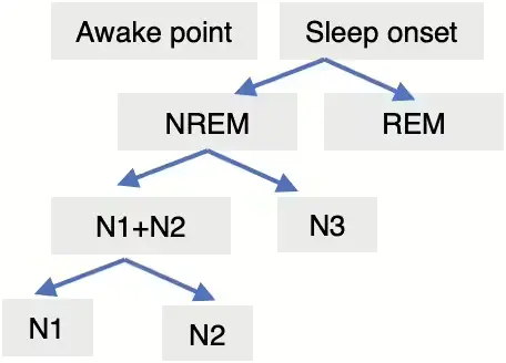
When it comes to detecting sleep stages, as confirmed in the research by Sundararajan et al.[5], the detection process is conducted in stages, as illustrated in the schematic diagram provided above in Figure 4. Initially perceived as relatively stable compared to activity may exhibit subtle fluctuations depending on the sleep stage, potentially leading to variations in body movement. Consequently, we hypothesized that enhancing the stability and consistency of the signal during the sleep period could facilitate the detection of sleep states.
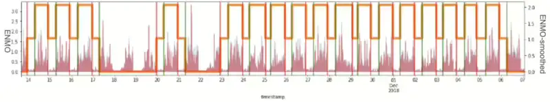
In attempting to improve the consistency of sleep signals, one straightforward approach is noise cancellation or filtering. The Power Spectral Density(PSD) is the method for finding the squared magnitude of FFT values, useful for understanding the distribution of power across different frequency bands. However, when utilizing Power Spectral Density (PSD) analysis, which is valuable for assessing the density ratio of FFT2 across various frequency bands, it was observed that this process unintentionally amplifies noise within the original sleep signal. Despite filtering out 0.2% of the total based on the analysis which means we are trying to leave the 99.8% signals without noise or outliers, the outcome distinctly contrasts with the initial intention of creating a more stable signal compared to the active period within the sleep phase. The schematic process equation 5 below describes the process applied for this purpose.
(5)[|f|]→FFT[|f^|]→|f^|2<99.8filter[|f^filter|]→inverseFFT[|ffilter|]
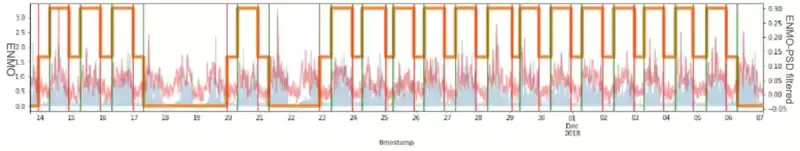
Figure 5 illustrates the resulting PSD graph as an example for one ID. Ultimately, instead of solely eliminating specific outliers from the entire density, it became apparent that updating the signal by incorporating information from previous time points was necessary. Recognizing the irregularity of signal noise, we employed the Kalman smoothing technique utilizing the covariance of previous data. The Kalman Filter is for tracking a single target in continuous state space. Given a sequence of noisy sleep measurements, the Kalman Filter can recover the “true state” of the underlying target being tracked. Consequently, we achieved the desired effect of filtering signals without compromising the integrity of the existing signal. However, it was observed that this approach was not entirely suitable for maximizing the stability of the sleep signal. Figure 6 illustrates the resulting Kalman smoothing graph as an example for one ID.
Considering that a typical day comprises 24 hours, the duration of sleep for most individuals is relatively shorter compared to their active periods and sometimes we can’t know which period belongs to which, because of missing labels. As a result, the data collected tends to exhibit an imbalance between the sleep and active segments. Therefore, when sampling from the sleep period to obtain consistent sleep signals, it becomes evident that the sampling process is inherently irregular.
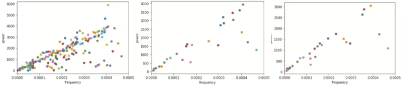
Hence, the Lomb-Scargle Periodogram[13] method was adapted to address this issue. This method is designed to detect and characterize periodic signals in unevenly sampled data. Unlike the PSD(Power Spectral Density), the periodogram has an unavoidable intrinsic variance, even in the limit of an infinite number of observations. While the Lomb-Scargle periodogram aims to extract periodic signals from irregularly sampled data, it’s essential to recognize that approaches such as cleaning may have inherent limitations. However, by cautiously applying this method on an ID-by-ID basis to the current data, we aim to avoid generating signals that significantly deviate from periodicity. Additionally, some collected data have no labels whether they represent sleep onset or wakeup onset, therefore the data is not enough to analyze periodicity, train data which made up 80% of Non-missing reports 35ea ID as a complete set, was used to apply in that case. In this experiment, five samples were extracted after each sleep interval, and another five samples were taken from the middle of each sleep interval to adjust the Lomb-Scargle Periodogram. After periodicity is found through 10 sample data per each sleep intervals of the entire sleep intervals. Among these, we sought to find the cycle with the highest power and remove this periodicity to create a stable sleep signal. Upon examining IDs without missing reports, if the dominant frequency exhibits linearity and the pattern appears consistent, it can be inferred that this approach is rational, as the frequency within the linear line reflects the effectiveness of this method.
Figure 7 illustrates the linearity of the dominant frequency. The left panel displays the results for a total of 269 IDs, the middle panel shows results for 35 IDs without missing reports and the right panel corresponds to 80% of the middle panel.
When applying the Lomb-Scargle periodogram, it’s crucial to comprehend the uncertainty associated with the determined frequency. In terms of periods, it’s common to observe a most significant amount of power around the period of approximately 1 hour. This occurrence aligns with the typical sleep cycle duration, making it a comprehensible result even when considering the currently sampled data. Figure 8 illustrates the Lomb-Scargle Periodogram applied result graph of 3ea sample ID respectively. (The first graph is for about 1 month duration, the second is for about 20 days, third graph is for about 25 days.)
In the processing workflow, when the number of samples does not extend beyond 3 to 5 days, significant data gaps often occur due to missing device data, which were addressed by applying a general dominant frequency approach.
However, when data for at least 3 days was available, a more individualized approach was adopted, considering each ID separately. Given the relatively longer duration of the cycle compared with the extremely short duration, the sleep period tends to appear relatively constant. Nonetheless, by not eliminating variability in this process, we aim to achieve the original objective of stabilizing a signal of a consistent pattern in a sleep period while minimizing information loss as much as possible.
3.2. Modeling
In this subsection 3.2 , we describe and provide a generalization method focused on sleep state detection, particularly utilizing distributions of sleep duration and active duration. By employing this duration’s distribution, a likelihood ratio comparison method is suggested between two different episodes. Typically, the distribution of the ENMO signal is not uniform for both sleep and active durations. Specifically, the distribution differs between these two episodes. A smooth envelope shape is often observed in the distribution of sleep episodes, whereas a sharp envelope shape is more common in the distribution of active episodes. This distinction in the distribution envelope shapes highlights the inherent differences between sleep and active periods in terms of their movement characteristics.


Figure 9 describes the density graph of raw ENMO signal and Figure 10 shows the density graph of signal processed(section 3.1 adjusted)ENMO for all IDs respectively. In Figure 9 and Figure 10, we can see that the peak value of the largest density of the processed signal does not differ significantly by ID in awake and sleep period.

After examining the distribution of all data points within both sleep and awake periods, without classification by ID, it was observed that the peak value of the entire dataset remains consistent when compared to the graph on the right, which represents 9% of the total data. This indicates stability in the peak value across different subsets of the data, reinforcing the reliability of the observed distribution patterns.


Figure 12. (a) : 80% data of complete set (about 9% of total data), (b) : resampling of (a) - sleep : active(awake) = 3185ea : 3135ea, (c) random sampling of (a): only data points with 786ea $\leftarrow$ train distribution data to be used only for initial input data.
We conducted several experiments to establish criteria for utilizing distribution data in future models. The graph labeled Figure 12 (a) consists of IDs with complete datasets containing without NaN values, and it represents a density graph utilizing only 80% of this data. Comparing it with Figure 11 which used a total dataset(consisting of 269ea ID), we observed a similar approximate shape. Through Figure 12 (b) and (c), we confirmed that random sampling and utilization of the data appear to be more appropriate. In essence, despite the relatively small number of data points, random sampling was employed to create a standardized distribution that better reflects the overall shape tendency. Through this, we wanted to use it as a train distribution when the initial input samples were insufficient. As shown in the distribution graph above, the distribution of sleep and awake periods may not fit the data well to the common density function (i.e., Gaussian, Poisson.. etc), and often the data distribution is irregular and it may not be similar to the common Probability Distribution Function (PDF). Therefore, the distribution was used by applying kernel density estimation. The kernel density estimation equation :
\begin{equation}\label{eq:kernel density estimation}
\hat{f}_{h}(x) = {1 \over n} \sum_{i=1}^{n} K_{n}(x-x_{i}) = {1 \over nh} \sum_{i=1}^{n} K({x-x_{i} \over h})
\end{equation}
The parameter $h$ is the kernel function of the bandwidth parameter. The kernel has a sharp shape (when $h$ is a small value), and the kernel has a smooth shape (when $h$ is a large value). In other words, for each observed data, a kernel function centered on the corresponding data value is generated :$(K(x - x_{i}))$. All kernel functions created in this way are added up and divided by the total number of data. Usually, the optimal kernel function is the Epanechinikov kernel, and for convenience of calculation, the Gaussian kernel is often used. In this paper, the Gaussian kernel is applied for computational efficiency. The data used in the distribution is about 800ea per distribution randomly (sleep episode, active episode). Now that the method for estimating the distribution has been explained, the next contents explain the entire model process. Following Figure 13 shows the whole process for state detection. We discussed signal processing in section 3.1. The detailed process rule is to randomly sample 800ea from the data created as train distribution data when the data does not exceed 3 days. As it is not appropriate to find sufficient periodicity for the initial new input data, the original signal was used.
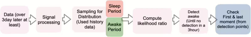
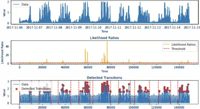
For the detection process, we employed previous data, utilizing a window of 4 days inclusive of new data. Additionally, when more than 3 days of data were available for each ID, we applied the methodology individually for each ID. This approach ensured a tailored and comprehensive analysis, considering the specific characteristics of each ID’s data. Here, this whole process proceeds sequentially from data input to final detection. In particular, the step of computing the likelihood ratio can be described by the following equation:
\begin{equation}\label{eq:LR}
LR = {L_{1}(D) \over L_{0}(D)}
\end{equation}
$L_{0}(D)$is the likelihood of the data under the null hypothesis(data is more likely sleep signal) and $L_{1}(D)$ is the likelihood of the data under the alternative hypothesis(data is more likely active signal). If the LR is greater than the threshold, it suggests that the data are more likely under the alternative hypothesis(active signal).
4. Results
In section 4, we describe the results of our main results and supplemental analysis. While there is no specific benchmark for comparison in this study, we’ve compared the original signal within the dataset used and verified the results using data that was not utilized in the model. This approach allowed us to assess the effectiveness and accuracy of our methodology by comparing results with both the original signal and unseen data.
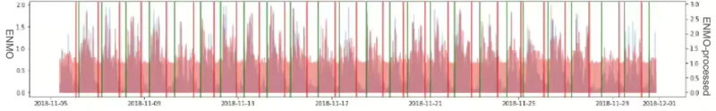
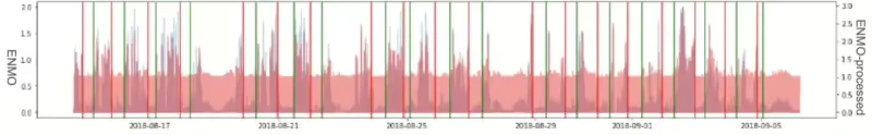
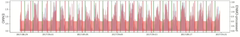
Figure 14 shows the result of applying the LR method for a specific 1 ID sample, in particular, we could check that the bottom graph of Figure 14 detects as many points in the active points including the first point of sleep onset and the last point of waking up.
As discussed earlier, we are utilizing kernel density estimation for distribution, and it’s crucial to consider computational costs. In the model process, data is transformed immediately upon input, and the likelihood ratio result is detected when it surpasses the threshold, leading to relatively fast calculation times. For instance, when computing approximately 39,059ea data points, it takes about 7 seconds. Therefore, in order to process a day’s worth of data for 10 people(approximately 17,280ea data points per person in one day), it would take a total of about 1 minute and 40 seconds. These results were obtained without using any additional computational skills, such as parallelization.
Finally, although it may seem obvious since distribution is utilized, we visually confirmed that our approach does not only identify non-wearing device points but also detects signals that are not non-wearing devices yet lack a corresponding label value in Figure 15 which is one of the result example of 1 ID. This highlights the effectiveness of our method in identifying such instances where label values are absent, contributing to a more comprehensive analysis of the data.

In this paper, we intend to use the time difference between the predicted value and the label value as a performance indicator. As a result of comparing the time difference between the model’s predicted value and the label value, there was a tendency to predict the time to fall asleep faster than the actual label value, and the overall tendency to predict the time to wake up slower than the actual label value. Hence, in order to check the cause of this issue, we applied the LR method to the original ENMO signal which means the signal is not processed to detect the sleep state. As the results can be seen in Figure 16 graph (a), the same fast and slow trends in prediction were confirmed even when using the original ENMO signal. The original signal must be used for the first three days, but Figure 16 (b) graph is the result using the fully processed ENMO signal for comparison. What is evident here is that the ENMO signal itself exhibits the mentioned tendency, and it can be observed that if the initial data is not collected for more than 3 days, signal processing leads to an increase in the variance of the prediction.
We confirmed the results of the model through standardized evaluation indicators for the time difference. The results of SE checks (Within individual Standard Error) for each ID are expressed as the average value of the within-individual standard error in table 1 and table 2. The results of randomly using 10ea IDs included in the Train distribution was displayed in train contained data(table 1), and the results of randomly using 3ea IDs not used in the Train distribution were displayed in test data(table 2).
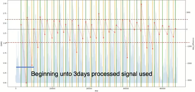
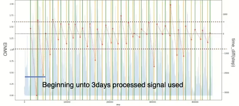
Figure 16. Time difference between model detected and label: (a) result graph of original signal utilized, (b) result graph of processed signal utilized (left y axis represents original ENMO signal and right y axis represents time difference. Additionally, green and yellow vertical lines describe awake and asleep moments in label data respectively. The predicted starting points of the vertical lines for both periods are shown in the lighter colour of each display colour.)
The scenario where the Train distribution is not used occurs when the ID itself has label values without omission, as seen in train contained data. Conversely, in the case of test data, NaN values exist in the label values, necessitating the use of the train distribution. These observations were confirmed through an examination using 3ea IDs not included in the train distribution. It was observed that the time difference standard error (S.E) value of the signal-processed data through data transformation decreased by more than 20 minutes in the test data compared to when the original signal was used. The results obtained for 13ea IDs, a total of approximately 110 days of nights, were checked by randomly extracting samples. Samples that were not used in the distribution were also randomly checked, indicating a high level of reliability in the data results.
\begin{array}{| p{4cm} | p{3cm} | p{3cm} |}
\hline
\textbf{train_contained_data} & \textbf{Original enmo} & \textbf{Processed enmo} \\
\hline
\text{S.E - wakeup(min)} & 37.62906 & 26.73768 \\
\text{S.E - sleep onset(min)} & 34.48122 & 26.59554 \\
\hline
\end{array}
Table 1. Detection standard error from IDs included in train distribution
\begin{array}{| p{4cm} | p{3cm} | p{3cm} |}
\hline
\textbf{test_data} & \textbf{Original enmo} & \textbf{Processed enmo} \\
\hline
\text{S.E - wakeup(min)} & 57.61296 & 21.55212 \\
\text{S.E - sleep onset(min)} & 56.40516 & 30.5604 \\
\hline
\end{array}
Table 2. Detection standard error from IDs excluded in train distribution
5. Conclusion
In our approach, we prioritized a generalized methodology over optimization. Utilizing raw signals increases dimensionality and can be significantly impacted by complexity by considering 3 axes depending on the base axis in the data. However, we improved efficiency through data transformation. Particularly, given the irregular properties of human sleep rules that are not always constant over time, we enhanced efficiency through signal processing using the Lomb-Scargle periodogram methodology, which can identify periodicity in irregularly sampled data. In particular, rather than utilizing the entire sleep period for signal processing, we used a small subset of data from a fairly stable period to make the signal more stable for the target sleep period.
Furthermore, by applying the likelihood ratio (LR) methodology compared to existing machine learning or deep learning models, we utilized a distribution with more information rather than point-wise fitting. This inevitably enhances efficiency as it provides more information than variance. Consequently, it becomes feasible to develop a more general model capable of accommodating initial values (provided there is data spanning more than 1 hour).
Additionally, the methodology presented offers higher computational efficiency compared to high-complexity models such as existing machine learning or deep learning approaches. Specifically, by comparing only the number of variables derived through existing rolling statistics, we were able to identify sleep state as one variable with a time difference with a median value of 1 hour.
Finally, the methodology presented features low model complexity, and the signal processing step and LR model method are performed sequentially at once, facilitating convenient modification of the model structure later on. This aspect may provide an advantage in terms of maintenance ease.
6. Discussion
In this paper, only the ENMO signal was utilized. However, given the consistent detection tendency of the signal and advancements in the field of actigraphy measurement with wearable devices, incorporating complementary variables such as heart rate could lead to more sophisticated state detection. By integrating accelerometer and pulse data, it is anticipated that state detection could become more refined.
Furthermore, from both modeling and data perspectives, performance enhancements are expected if detailed updates are made during signal processing for each ID. In our study, we conducted a simple experiment to determine the period during which historical distribution data could be utilized or the dominant frequency. However, it may be possible to consider making precise adjustments in the future.
Additionally, we observed characteristic groups existing by ID (between individuals), suggesting that in future research, dividing each ID into extreme groups (i.e., groups with above-average activity vs. groups with little activity) could simplify threshold adjustments and potentially improve accuracy. This observation was included in section 7.
Expanding the study group beyond the scope of this research could contribute significantly to public healthcare research by reflecting the demographic characteristics of people in terms of business or sleep research. This broader perspective could offer valuable insights into population health trends and facilitate more targeted interventions and policies.
7. Additional contents
We found out that the individual signal characteristic was different in Figure 17.
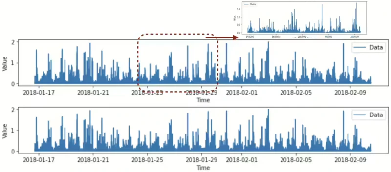
Figure 17. Signal characteristics of two different groups.
References
[1] Jiawei Bai, Chongzhi Di, Luo Xiao, Kelly R. Evenson, Andrea Z. LaCroix, Ciprian M. Crainiceanu, and David M. Buchner. An activity index for raw accelerometry data and its comparison with other activity metrics. PLOS ONE, 11(8):1–14, 08 2016. doi: 10.1371/journal.pone.0160644. URL https://doi.org/10.1371/journal.pone.0160644.
[2] Kishan Bakrania, Thomas Yates, Alex V Rowlands, Dale W Esliger, Sarah Bunnewell, James Sanders, Melanie Davies, Kamlesh Khunti, and Charlotte L Edwardson. Intensity thresholds on raw acceleration data: Euclidean norm minus one (enmo) and mean amplitude deviation (mad) approaches. PloS one, 11(10):e0164045, 2016.
[3] Roger J. Cole, Daniel F. Kripke,William Gruen, Daniel J. Mullaney, and J. Christian Gillin. Automatic sleep/wake identification from wrist activity. Sleep, 15(5):461–469, 09 1992. ISSN 0161-8105. doi: 10.1093/sleep/15.5.461. URL https://
doi.org/10.1093/sleep/15.5.461.
[4] Aiden Doherty, Dan Jackson, Nils Hammerla, Thomas Pl¨otz, Patrick Olivier, Malcolm H. Granat, Tom White, Vincent T. van Hees, Michael I. Trenell, Christoper G. Owen, Stephen J. Preece, Rob Gillions, Simon Sheard, Tim Peakman, Soren Brage, and Nicholas J. Wareham. Large scale population assessment of physical activity using wrist worn accelerometers: The uk biobank study. PLOS ONE, 12(2):1–14, 02 2017. doi: 10.1371/journal.pone.0169649. URL https://doi.org/10.1371/journal.pone.0169649.
[5] Sundararajan K., Georgievska S., B.H.W. te Lindert, Philip R. Gehrman, Jennifer Ramautar, Diego R. Mazzotti, Sabia S´everine, Weedon Michael N., van Someren Eus J. W., Ridder Lars, Wang Jian, and van Hees Vincent T. Sleep classification
from wrist-worn accelerometer data using random forests. Scientific Reports, 11(1):1–24, 01 2021. doi: 10.1038/s41598-020-79217-x. URL https://doi.org/10.1038/s41598-020-79217-x.
[6] Marta Karas, Jiawei Bai, Marcin Str´aczkiewicz, Jaroslaw Harezlak, Nancy W. Glynn, Tamara Harris, Vadim Zipunnikov, Ciprian Crainiceanu, and Jacek K. Urbanek. Accelerometry data in health research: challenges and opportunities. bioRxiv, 2018. doi: 10.1101/276154. URL https://www.biorxiv.org/content/early/2018/03/05/276154.
[7] Miguel Marino, Yi Li, Michael N. Rueschman, J. W. Winkelman, J. M. Ellenbogen, J. M. Solet, Hilary Dulin, Lisa F. Berkman, and Orfeu M. Buxton. Measuring sleep: Accuracy, sensitivity, and specificity of wrist actigraphy compared to polysomnography. Sleep, 36(11):1747–1755, 11 2013. ISSN 0161-8105. doi: 10.5665/sleep.3142. URL https://doi.org/10.5665/sleep.3142.
[8] Jairo H Migueles, Alex V Rowlands, Florian Huber, S´everine Sabia, and Vincent T van Hees. Ggir: a research community–driven open source r package for generating physical activity and sleep outcomes from multi-day raw accelerometer data. Journal for the Measurement of Physical Behaviour, 2(3):188–196, 2019.
[9] Nigel R Oakley. Validation with polysomnography of the sleepwatch sleep/wake scoring algorithm used by the actiwatch activity monitoring system. mini mitter co. Sleep, 2:0–140, 1997.
[10] Joao Palotti, Raghvendra Mall, Michael Aupetit, Michael Rueschman, Meghna Singh, Aarti Sathyanarayana, Shahrad Taheri, and Luis Fernandez-Luque. Benchmark on a large cohort for sleep-wake classification with machine learning techniques. npj Digital Medicine, 2(1):1–9, 06 2019. doi: doi.org/10.1038/s41746-019-0126-9. URL https://doi.org/10.1038/ s41746-019-0126-9.
[11] Vincent T. van Hees, Lukas Gorzelniak, Emmanuel Carlos Dean Le´on, Martin Eder, Marcelo Pias, Salman Taherian, Ulf Ekelund, Frida Renstr¨om, Paul W. Franks, Alexander Horsch, and Søren Brage. Separating movement and gravity components in an acceleration signal and implications for the assessment of human daily physical activity. PLOS ONE, 8(4):1–10, 04 2013. doi: 10.1371/journal.pone.0061691. URL https://doi.org/10.1371/journal.pone.0061691.
[12] Vincent Theodoor van Hees, Severine Sabia, Samuel E Jones, Andrew R Wood, Kirstie N Anderson, M Kivim¨aki, Timothy M Frayling, Allan I Pack, Maja Bucan, MI Trenell, et al. Estimating sleep parameters using an accelerometer without sleep diary. Scientific reports, 8(1):12975, 2018.
[13] Jacob T VanderPlas. Understanding the lomb–scargle periodogram. The Astrophysical Journal Supplement Series, 236(1):16, 2018.
[14] Henri Vähä-Ypyä, Tommi Vasankari, Pauliina Husu, Jaana Suni, and Harri Siev¨anen. A universal, accurate intensity-based classification of different physical activities using raw data of accelerometer. Clinical Physiology and Functional Imaging, 35(1):64–70, 2015. doi: https://doi.org/10.1111/cpf.12127. URL https: //onlinelibrary.wiley.com/doi/abs/10.1111/cpf.12127.