Price Premium Discovery In Real Estate Auction Market: Decomposition Of The Korea Auction Sale Rate

Price Premium Discovery In Real Estate Auction Market:
Decomposition Of The Korea Auction Sale Rate

Bohyun Yoo

1. Introduction

The housing auction market in Korea is one of the real estate markets, and many stakeholders such as mortgage banks, arbitrage investors, and non-performing loan operators are deeply involved. In general, there is a perception that the auction market is surcharged or discounted compared to the general market. If the auction market is an efficient and fair-trading market, it will not be different from the general market price, but most housing auction cases are implemented by default, so it is known that have legal issues and that applies as a discount factor. However, the bottom-up analysis based on individual auction cases, which is a method mainly used in previous studies on discounts and surcharges, is limited in time and space, and the time-varying effect cannot be considered, and the results of the analysis are limited and dependent on the data held by the researcher.

To overcome these limitations, it should be carried out the analysis from the market perspective, but the time series data Auction Sale Rate is unreliable as an indicator because the court appraiser price, which is the standard, is performed at the past rather than at the time of the auctioned price. It is difficult to specify the time of court appraisal as a variable in the model because it varies from case to case of individual auction how much it is in the past at the time of successful bid, and even if the time is known, the court appraisal price cannot be accurately estimated. Individual cases can be investigated in a bottom-up manner to return the point of view based on the general market price, but it is a very vast task and likewise a study limited to time and space.

The target of this paper is the apartment auction market, and to overcome the limitations of the auction sale rate, the auction sale rate is decomposed into three components in a top-down manner using Fourier transform. The proof of the decomposed each component is performed. And the price premium effect at the auction market is presumed and the reason is analyzed and the section discrimination in which the price premium effect acts is attempted. In addition, the time-varying beta through the Kalman filter is used to support the price premium effect, and the analysis of how the price premium effect differs in each region’s market is also performed.

2. Literature review

Shilling et al (1990) analyzed the apartment auction in 1985 in the baton lounge, Louisiana, USA, and found an auction discount rate of -24%, Forgey et al (1994) analyzed houses from 1991 to 1993 in the United States and found that they were traded at a -23% discount. Spring (1996) analyzed foreclosures in Texas from 1991 to 1993 and found a 4-6% discount, Clauretie and daneshvary (2009) analyzed the housing auctions from 2004 to 2007 and found that about 7.5% of foreclosures were discounted because of endogenous and autocorrelation.

Campbell et al (2011) analyzed about 1.8 million housing transactions in Massachusetts and found that the discount rates for foreclosures and deaths were different. Zhou et al (2015) found that on average, 16 cities in the United States were discounted by 14.7%, Arslan, Guler & Tasking (2015) analyzed that a 1% increase in risk-free interest rates led to a 27% drop in house prices and a 3% increase in foreclosure rates.Jin (2010) compared and analyzed the general sale price and the auction price of apartments in Dobong-gu, Seoul and Suji-gu, Yongin-si, Korea, and found that the auction price is more discounted than the general transaction price. Lee (2012) noted that the real estate market is not efficient and is one of the anomalies of the discount / surcharge phenomenon in the apartment auction market.

Lee (2009) and Oh (2021) pointed out the limitations that occurred when the court appraisal price and the auctioned price were different and estimated the auction sale rate by correcting the court appraisal price to the auctioned time.

However, previous studies mainly focus on the analysis of variables in the bottom-up method along with the limitation of space and time based on individual auction cases. In addition, it is difficult to see the analysis in the same environment as Korea because the cases other than Korea adopt the open bidding system.

3. Materials and method

3.1. Decomposition of auction sale rate

Configuration of the auction sale rate defined as

\begin{equation} \label{eq:auction-sale-rate}
Auction\ Sale\ Rate\ _t=\frac{\sum_{i}\ Auctioned\ Price_{it}}{\sum_{i}\ Appraisal\ Price_{it-n}}\
\end{equation}

\begin{equation} \label{eq:auction-price}
Auctioned\ Price_t=\ Market\ Price_t\pm\ Price\ Premium_t\ (=discount\ or\ surcharge)
\end{equation}

\begin{equation} \label{eq:auction-sale-rate-price}
Auction\ Sale\ Rate\ _t=\frac{\sum_{i}\ (Market\ Price_t\ \pm\ Premium\ _t)}{\sum_{i}\ Appraisal\ Price_{t-n}}
\end{equation}

\begin{equation} \label{eq:market-price}
\text{If}\ Price\ Premium_t=0\ ,\ \ Market\ Price_t=Auctioned\ Price_t
\end{equation}

Where i is each auction case, t is each per month. If the auctioned price is discounted and surcharged compared to the general market price, the component can be separated as shown in (2), and if there is no discount and surcharge, it can be expressed as shown in (4). In order to estimate the price premium effect, which is the discount or surcharge, it can be defined in the Regression form as shown in (5), and it is assumed that the explanatory power of each component is as shown in (6).

In the Regression form in terms of effects,

\begin{equation} \label{eq:auction-sale-rate-in-regression}
Auction\ Sale\ Rate\ _t={\beta_0}_t{+\beta}_1EoM+\beta_2EoA_t+\ \beta_3EoP_t+\epsilon_t
\end{equation}

\begin{equation} \label{eq:explanatory-power}
\text{Explanatory Power of Each Components :} \\
EoM (Effect of Market Price) > EoA (Effect of Appraisal Price) > EoP (Effect of Price Premium)
\end{equation}

3.2. The data

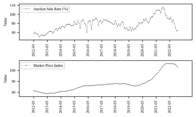
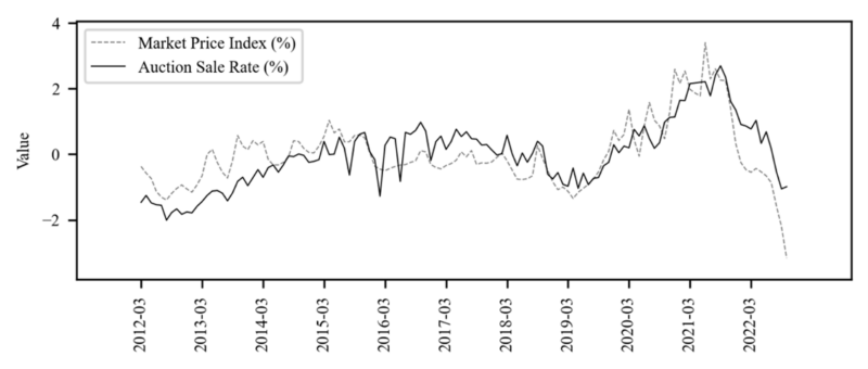
The empirical analysis in this paper is based on Auction Sale Rate and Market Price Index in nationwide 2012.03 ~ 2022.10 in month. The auction sale rate is calculated by collecting the sum of court appraiser prices and auctioned prices nationwide announced by the court from 2012.03 to 2022.10. The Market price index is an index of general market apartment prices nationwide and is provided by the Korea Real Estate Board. Log-Differencing is taken in the Market price index to match the forms of both data equally then Standardization, which translates to mean 0 and variance 1, take both data to match the same scale.

skewness and kurtosis reported in Table 1 shows AuctionSaleRate and MarketPriceIndex has different peaks and tails compared to normal distribution. and the Lev results in Table 1 show that it is different from the leverage effect (Black 1976.) of the stock market. The auction market and the general sales market has a positive sign relationship with the future volatility. This means that volatility in the real estate market has a positive correlation with price.

3.3. Identification of variables

3.3.1. The effect of market price

Auction sale rate can be decomposed into three components in the regression form as shown in (5), and log-differencing market price index is used as the first variable, EoM’s proxy variable. As shown in Table 2, EoM has the strongest explanatory power in auction sale rate.

3.3.2. Component identification

\begin{equation} \label{eq:component-identification}
y_t=\beta_0+\beta_1Mkt_t+\epsilon_t
\end{equation}

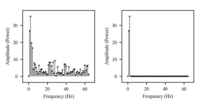
Where y_t is Auction sale rate at time t, $\beta_0$ is intercept $\beta_1$ is parameter of $Mkt$ and $Mkt$ is Log differencing Market Price Index. as define in (5), the remaining EoA and EoP components are in the residual as latent. To identify EoA, EoP components, a Fourier transform is used in $\epsilon_t$ (7), and then two highest amplitude signals can be extracted, assuming that they are court appraisers and price premium effects as defined in (6).

3.3.2.1. Fourier transform

Fourier transform is a mathematical transformation that decomposes a function into a frequency component, representing the output of the transformation as a frequency domain. In this paper, it is used to extract the orthogonal cycle of EoA and EoP as defined in (5). In terms of linear transformation, the orthogonal factor present in the signal can be extracted as a Forward and Inverse Discreate Fourier matrix, as shown in (9).

\begin{equation} \label{eq:fft}
X=F_{N}x \ \text{and} \ x=\frac{1}{N}F_N^{-1}X\ \text{<Forward and Inverse>}
\end{equation}

\begin{equation} \label{eq:fft-in-matrix}
{\underbrace{\left[\begin{matrix}
X\left[0\right] \\
X\left[1\right] \\
\vdots \\
X\left[N-1\right] \\
\end{matrix}\right]}}_{Signal} \
= \
{\underbrace{\left[\begin{matrix}
W_N^{0\cdot0} & W_N^{0\cdot1} & \cdots & W_N^{0\cdot(N-1)} \\
W_N^{0\cdot1} & W_N^{0\cdot1} & \cdots & W_N^{1\cdot(N-1)} \\
\vdots & \vdots & \ddots & \vdots \\
W_N^{0\cdot1} & W_N^{0\cdot1} & \cdots & W_N^{(N-1)\cdot(N-1)} \\
\end{matrix}\right]}}_\text{$F_N$(Discrete Fourier Matrix)} \\
{\underbrace{\left[\begin{matrix}
x\left[0\right] \\
x\left[1\right] \\
\vdots \\
x\left[N-1\right] \\
\end{matrix}\right]}}_\text{Residual($\epsilon_t)$} \\
\text{, where } W^{n\cdot k}=\exp{\left(-j\frac{2\pi k}{N}n\right)}
\end{equation}

\begin{equation} \label{eq:signal-k}
X\left[k\right]=x\left[0\right]W^0+x\left[1\right]W^{N\times1}+\ldots+\ x\left[n-1\right]W^{i\times\left(n-1\right)} , \text{where} \ k=signal_k
\end{equation}

where $x$ is vector of $\epsilon$ in (7) $x=\left(x_0,x_1\ldots x_N\right)^T$ $N$ is length of vector and $X$ is signal $X=\left(X_0,X_1\ldots X_N\right)^T$ and $F_N$ is Discrete Fourier Matrix. As shown (9), (10) time series data which cyclic can be decomposed to orthogonal signal by Discrete Fourier Transform as linear transformation. However, in practice, DFT calculation $O(N^2)$ are replaced by Fast Fourier Transform (Cooley-Tukey algorithm, 1965) which is that performs fast calculations by dividing the DFT into odd and even two terms. $O\left({Nlog}_\ N\right)$ (11). Figure 3 shows that two high amplitude signals were extracted by performing FFT on Residual in (7).

\begin{equation} \label{eq:n-log-n}
\begin{split}
X\left[ k \right] & = \sum_{n=0}^{N-1} x_n \ exp \left( -j \frac{2 \pi k}{N} n \right) \\
& = \sum_{m=0}^{N/2-1}x_{2m}\exp{\left(-j\frac{2\pi k}{N}2m\right)}+\ \sum_{m=0}^{N/2-1}x_{2m+1}\exp{\left(-j\frac{2\pi k}{N}2m+1\right)} \\
& = \sum_{m=0}^{N/2-1}x_{2m}\exp{\left(-j\frac{2\pi k}{N\ /\ 2}\ m\ \right)}+\exp{\left(-j\frac{2\pi k}{N}\ \right)}\sum_{m=0}^{N/2-1}x_{2m+1}\exp{\left(-j\frac{2\pi k}{N/2}m\right)}
\end{split}
\end{equation}

where $x_{2m}=(x_0,x_1\ldots\ x_{n-2})$ is even-indexed part, $x_{2m+1}=(x_1,x_3,\ldots,x_{n-1})$ is odd-indexed part.

3.3.2.2. Regression analysis

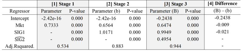
\begin{equation} \label{eq:stage-2}
Y_t=\beta_0+\beta_1Mkt_t+\beta_2SI{G1}_t+\mu_t
\end{equation}

\begin{equation} \label{eq:stage-3}
Y_t=\beta_0+\beta_1Mkt_t+\beta_2SI{G1}_t+\beta_3\widehat{SIG2_t}+\omega_t
\end{equation}

\begin{equation} \label{eq:signal-2}
\widehat{Sig2_t}=\sigma\left(Sig2_t\right) , \ \sigma=\frac{1}{1+e^{-\left(x\right)}} , \ >\ 0.5\ =\ 1\ \ ,\ <0.5=\ 0
\end{equation}

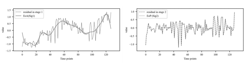
where $SIG1$ is highest amplitude signal in residual in $\epsilon_t$ (7) and $SIG2$ is highest apmplitude signal residual in $\mu_t$ (12)

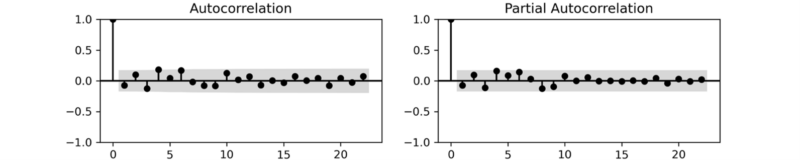
Table 2 shows the results of using the extracted signals as a variable of regression by performing FFT in 4.3.2.1. $SIG2$ is a component of EoP, and to distinguish price premium effects clearly, it is transformed into categorical data(0/1) through Sigmoid function as shown in (14). The Difference result in Table 2 show that the parameter has hardly changed, demonstrating that the two signals found are almost orthogonal components, and do not make omitted variable bias(Wooldridge, 2009). and the adj. R-squared supports the order of explanatory power assumed in (5). Lastly, the residual ACF/PACF plot in Figure 4 indicates that no further patterns exist in the residuals following the exclusion of the three components. (13) This supports the assumption outlined in 3.1 (5) that the auction sale rate is composed of three main components.

3.3.3. Proof of the effect of appraisal price

Based on Table 2 and according to the assumption of (5), $SIG1$ is EoA (Effect of Appraisal Price in Auction Sale Rate). The court appraisal time is in the past rather than the Auctioned time (1). The difference between the two points makes it difficult to define the court appraiser effect variable in terms of time series analysis. Since correcting the price difference that occurred in time for all auction cases is a very difficult challenge, the Fourier transform (4.3.2.1) is used. In this paper. Proving that $SIG1$ is EoA, 2,762 individual auction cases occurred between 2016.04 and 2018.03 in Seoul and Busan are empirically analyzed (Table 3, Table 4.)

The analysis is conducted in two main aspects:

1. Time interval between the time of court appraisal and the time of Auctioned (Table 4)
2. Regression with the general market price at the time of court appraisal price (Table 4)
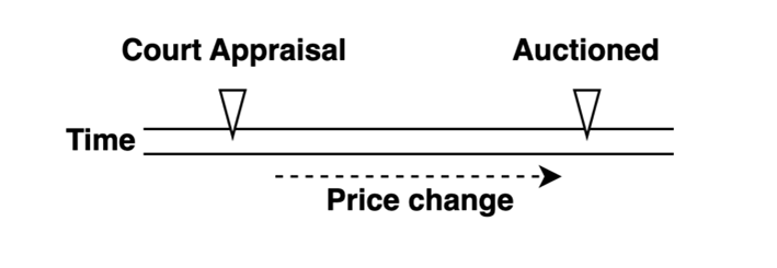
   \begin{equation} \label{eq:cp}
   CP_t=\ \alpha_0dummy_t+\alpha_1MP_t+\gamma_t
   \end{equation}

where $CP_t$ is price at time of court appraisal (Figure 5), MP is housing price, $\alpha_0$ is dummy variable $\alpha_1$is parameter of housing price.

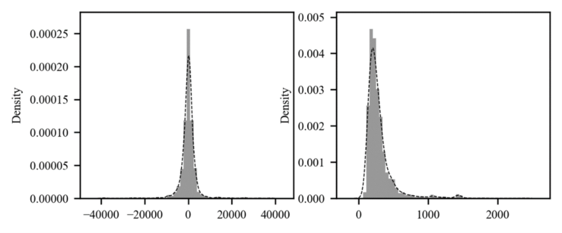
As shown in Table 4, the time difference distribution has a right skewed shape and the range of 25% to 75% is about 7 to 11 months. Price difference has a long-tailed distribution, and it can be estimated that the court appraisal price and the housing price at the time of the court appraisal have a very high correlation and are almost the same value. To summarize the results of the two analyses, the court appraisal price is the lag variable of the housing price. In terms of the component (5) EoA can be assumed to have a lag relationship with $Mkt$ and the results are shown in Table 5.

Table 5 [1] shows the relationship between the lag variable of $SIG1$ and $Mkt$. $SIG1$ extracted by Fourier transform is compared with lag variable and $Mkt$ of $SIG1$ because it is a signal indicating the past influence of the present time rather than the past price itself. In addition, the order of the Lag of the comparison target is set from 7 months to 11 months, which ranges from 25% to 75% of Table 4 As a result of the analysis, it was confirmed that the lag variable of $SIG1$ has a significant relationship with $Mkt$.

Table 5 [2] is a confirmation of whether $Mkt$’s lag variable can replace the court appraiser if the court appraisal price has a time lag relationship with the $Mkt$ according to the results of Table 4 As a result of the analysis, there is a significant relationship.

Table 5 [3] confirms the relationship between $SIG1$ and Auction sale rate. If the court appraiser can be replaced by $Mkt$’s lag variable only, as in Table 5, the $SIG1$ variable is not meaningful, but the results of the analysis show that Table 5 [3] is superior to Table [2]. The reason for this is that, as in Figure 6, there is no special depreciation factor in each auction case, which can be explained by $Mkt$’s lag, but there is an unidentified area that has a large gap with $Mkt$, such as legal issues, equity auctions, or the time difference does not fall between 25% and 75%.

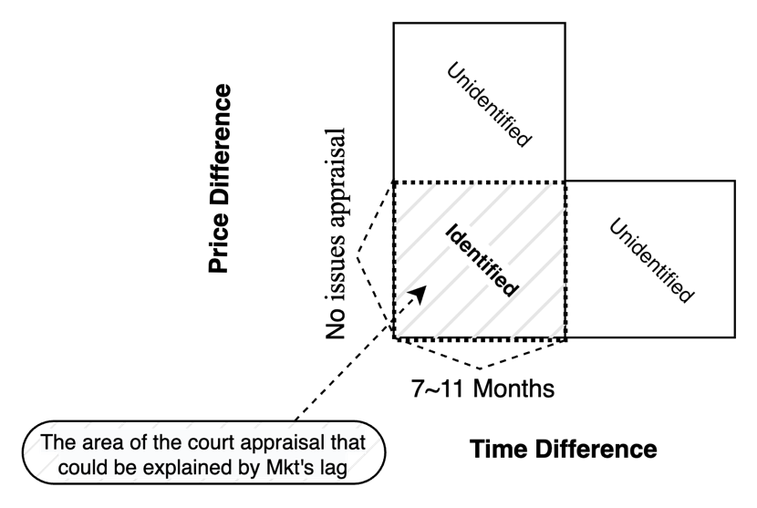
To sum up with Result of Table 5, in Table 4 $Mkt$ and $SIG1$ have lag relations with $Mkt$ and are superior to the lag variables of $Mkt$ according to the limits of Figure 7. therefore, $SIG1$ can be presumed in terms of EoA, as assumed in (5).

3.3.4. Proof of the effect of premium price

Based on result of Table 2 and according to the assumption of (5), $SIG2$ is EoP (Effect of Price Premium in Auction Sale Rate). For the analysis, $SIG2$ is transformed to categorical value through sigmoid function to assume Price premium on/off as in 4.3.2.2. In this paper, two aspects support that $SIG2$ is an EoP.

1. Verify that $\widehat{SIG2}$ can distinguish between discount and surcharge points. (Figure 8)
2. Track what variables $SIG2$ is, name it, and verify it makes sense.

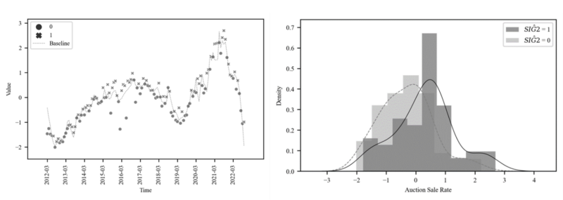
3.3.4.1. Distinguish to price premium pffect in auction sale rate

The $\widehat{SIG2}$ parameter of Table 2 [3] is about 0.49 with a positive sign Figure 8 is based on the baseline predicted by Table 2 [2], and the auction sale rate points are clearly distinguished up and down by $\widehat{SIG2}$ 1/0 of Table [3]. The righthand side of Figure 8 shows a distribution of different means and variances. Therefore, $SIG2$ can be presumed in terms of EoP, as assumed in (5).

3.3.4.2. Momentum factor

In 4.3.4.1, it is confirmed that $SIG2$ is a component that can explain the price premium effect, but it is meaningless if it cannot be explained by any variable in practice. In this paper, $SIG2$ confirms which variables can be compared, verifies whether it makes sense, and finally names it. First, $SIG2$ is likely to be a variable of the auction market itself because it is likely that EoM and EoP already has the effects of macro in almost. In fact, no significant correlation was found between comparable macroeconomic variables. According to the Lev result of Table 1, the future volatility of the auction market has a positive correlation with the auction sale rate, The EoP component also has a positive correlation according to table 2 [3]. So, the variable that can be compared as a component of the auction market itself is volatility (16)(17). The results of the verification of this hypothesis is shown in Table 6.

\begin{equation} \label{eq:signal-2-2}
SIG2_t=\ c_0+c_1{v1}_t+c_2{v2}_t+\eta_t, \ {v1}_t = \left(y_t-y_{t-1}\right)_t , \ {v2}_t=\ \left(y_{t-1}-y_{t-2}\right)_t
\end{equation}

\begin{equation} \label{eq:signal-2-3}
SIG2_t=\ c_0+c_1\left(y_t-y_{t-1}\right)t+c_2\left(y{t-1}-y_{t-2}\right)_t+\eta_t
\end{equation}

where c_0 is intercept, y is auction sale rate, v is volatility as differencing of auction sale rate.

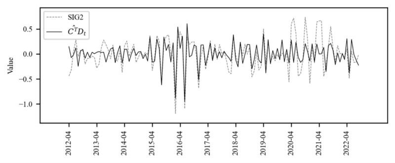
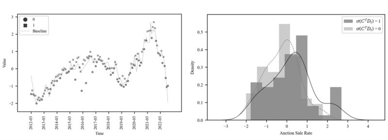
In Table 6, the volatility variable is significantly related to $SIG2$, and in Table 6, the value described by
the volatility variable (16)(17) and $SIG2$ show similar movements. Figure 10 shows that the volatility variable can distinguish between the surcharge and discount points well and has different distribution like Figure 8.

In summary, the volatility variable of Auction sale rate can be explained as the main factor that creates the Price premium effect, and in particular, the reason why volatility causes the price premium effect can be interpreted as the reason that the volatility of the auction market has a positive correlation with the Auction sale rate. As a result, the volatility component can be named the momentum of the auction market.

3.3.5. Time varying beta to capture price premium section

In 4.3.4, it was confirmed that $SIG2$ extracted through Fourier transform is a price premium effect and verified that it is a momentum factor. However, the analysis period of this paper is about 10 years, and it would be more reasonable to assume time-varying than parameter between the market and the Price Premium variable has a fixed constant. It means that the $\beta s$ (18) is not stable over time. Sensitivity of beta can be used to capture the section where momentum works in the market, beyond simply distinguishing the effect of price premium. In this paper, a Kalman filter is used to estimate the time-varying beta and Kalman filter is used to estimate the time-varying parameter.

\begin{equation} \label{eq:betas-not-stable}
{y_t=\beta_0}_\ {+\beta}_1Mkt_t+\beta_2SIG1_t+\ \beta_3\ {\widehat{SIG2}}_t+\epsilon_t , \epsilon_t~N(0,\sigma^2)
\end{equation}

3.3.5.1. Kalman filter

The Kalman filter is a model for describing dynamics based on measurements and recursive procedure for computing the estimator of the unobserved component or the state vector at time t.

\begin{equation} \label{eq:state-model}
\xi_t=F_t\xi_{t-1}+q_t , q_t~N(0,Q_\ ) \ \text{<State Model>}
\end{equation}

\begin{equation} \label{eq:observation-model}
y_t=H_t\xi_t+r_t , r_t~N(0,R_\ ) \ \text{<Observation Model>}
\end{equation}

<Predict Step>

Calculate the optimal parameter of $\xi_{t|t-1}$, based on available information up to time $t-1$,

\begin{equation} \label{eq:xi-hat}
{\hat{\xi}}{t|t-1}=F_t{\hat{\xi}}{t-1|t-1}
\end{equation}

\begin{equation} \label{eq:covariance-xi}
P_t=F_tP_{t-1}F_t^T+Q_\
\end{equation}

\begin{equation} \label{eq:state-matrix}
F_t=H_tP_{t-1}H_t^T+R
\end{equation}

Calculate the optimal parameter of $\xi_{t|t}$, based on available information up to time $t$,

\begin{equation} \label{eq:kalman-gain}
K_t=P_{t|t-1}H^T{F_{t|t-1}^T}^{-1}
\end{equation}

\begin{equation} \label{eq:covariance-at-time-t}
P_{t|t}=\left(1-K_tH_t\right)P_{t|t-1}
\end{equation}

\begin{equation} \label{eq:xi-at-time-t}
{\hat{\xi}}{t|t}={\hat{\xi}}{t|t-1}-K_t\ r_{t|t-1}\
\end{equation}

The random walk effect is considered by assuming that Q, R is the initial value near 0 (= diffuse prior) and F is the diag (1,1,1,1) unit matrix and the Kalman gain (K) determines the weight for the new information using the information of the error between the prediction and the observation.

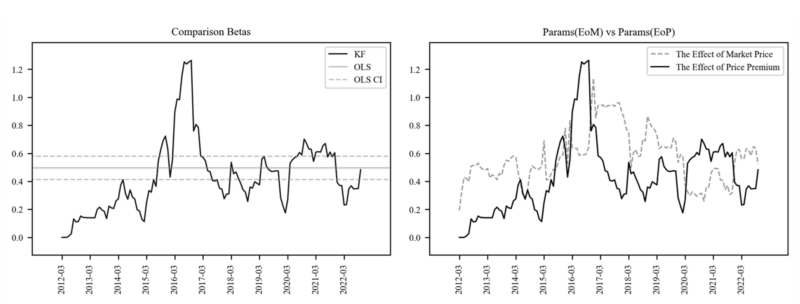
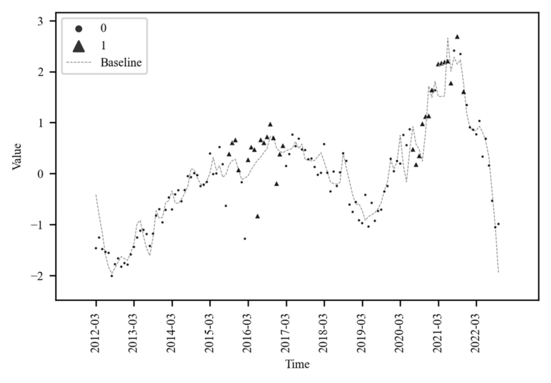
Table 8 shows that Time varying betas with Kalman filter performs better than the OLS with stable parameters. Figure 11 compares the change of the parameters of $\widehat{SIG2}$ and the change of the parameters of $Mkt$ at the same time. In Figure 12, if the parameter of $\widehat{SIG2}$ exceeds the upper confidence interval of OLS, it is set to 1 and plotted. In Figure 11, the area where $\widehat{SIG2}$ exceeds the beta of $Mkt$ and the area 1 of Figure 12 are the same, indicating that the price premium effect of the
auction market is more sensitive than the market price effect. This can be assumed to be an momentum interval, and the price premium effect is a sensitive interval.

3.3.5.2. Experiment

It is necessary to confirm whether the logic constructed so far works in the auction market in the region other than the whole country. Furthermore, when the model is performed by region, the characteristics of each region can be confirmed. The target areas of the empirical analysis are Seoul and gyeong-gi area where the auction market is most active.

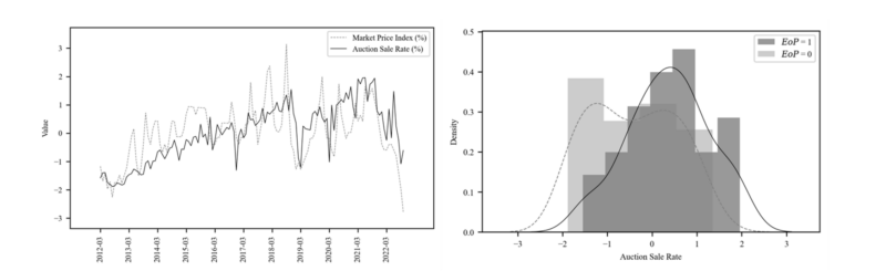
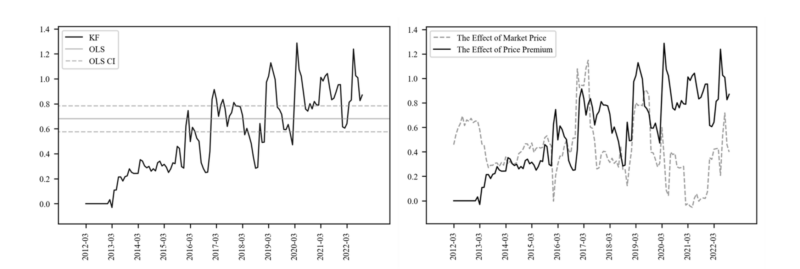
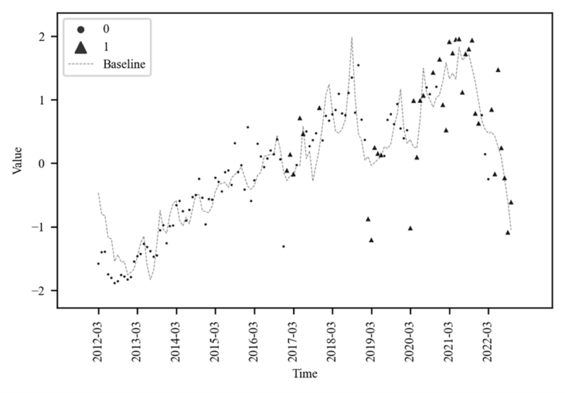
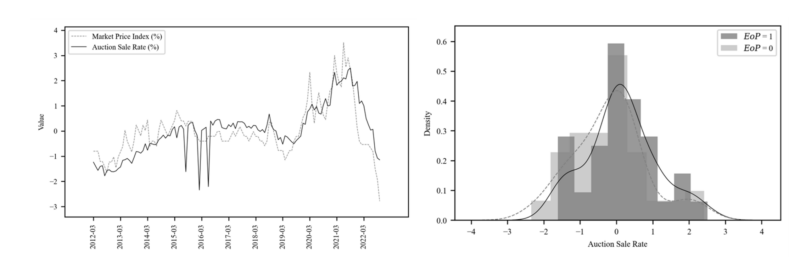
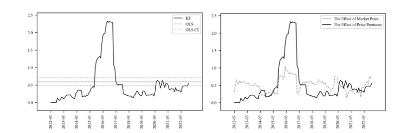
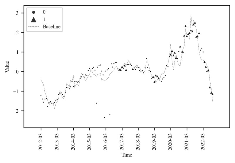
Table 8 and Figure 13 to Figure 18 are the results of the analysis of Seoul and Gyeonggi Province. Table 8 [2] Beta of $SIG2$ shows that Seoul is a more sensitive area than Gyeonggi-do in terms of price premium, and Figure 13-15 shows these resultswell. In particular, Seoul’s Beta of EoP has far exceeded $Mkt$’s Beta since early 2020, supporting the general perception that overheating sentiment is forming in the Seoul area in the apartment auction market. On the contrary, the effect of EoP is relatively low in Gyeonggi-do. In addition, through the above results, it can be distinguished whether the outlier points existing in the auction sale rate of each region are the influence of EoP.

4. Conclusion

The previous auction market studies using bottom-up method mainly analyzed the variables affecting the Auction sale rate or had the disadvantage that the space and time were limited to the data they had. In this paper, time series analysis was carried out from the market perspective, and the top-down method using Fourier transform was attempted to solve the problem that the court appraiser price could not reflect the general market price at the time of the auction, and the price premium effect could be specified through the proof of each component.

In addition, it was found that the reason for making the price premium effect in the auction market is the momentum effect, and the time varying beta (Kalman filter) supports the above logic showing that the price premium effect can be divided by region. It is practically impossible to analyze a vast amount of auction cases for the analysis of the auction market, and this paper was very encouraging in that it provided many participants in the auction market with indicators that can be viewed from a market perspective.

However, it requires a deep understanding of the momentum factor. The sensitive activity of the momentum factor signifies not just market rises or falls, it indicates shifts in the price relationship between the auction and the general markets. Intuitively, when the real estate market heats up, high demand narrows the gap between general market prices and auction prices.

Therefore, the role of the momentum factor can be interpreted as representing the ‘popularity’ of the auction market compared to the general market. To elaborate further, it can serve as an indicator to judge whether the market is overheating or cooling down in comparison to the general market.

The additional insights of this study are as follows: Korea’s apartment auction market has only momentum factors except for market prices under court appraiser control. Macro factors such as government regulations and interest rates are in the market price, so the third variable of the auction market is only the momentum factor, which can be very important information for many participants in the auction market.

This paper can be more rigorous if the following limitations are resolved. Since the monthly auction sale rate data may not be enough to support the rigor of the analysis, a wider analysis period or more time will further support the rigor of the analysis. In addition, the rigor of the analysis will be supported if more data on the unidentified area can be obtained in the process of proving the appraiser component of the court.

References

[1] Arslan, Y., Guler, B. & Taskin, T(2015), “Joint dynamic of house prices and foreclosures,”

[2] Journal of Money, Credit and Banking, 47(1), 133-169.

[3] Clauretie, T.M., Daneshvary, N.,(2009). “Estimating the house foreclosure discount corrected for spatial price interdependence and endogeneity of marketing time,” Real Estate Economics. 37 (1), 43-67.

[4] Campbell, J.Y., Giglio, S., Pathak, P.,(2011). “Forced sales and house prices,” American Economic Review. 101 (5), 2108-2131.

[5] Forgey, F.A., Rutherford, R.C., VanBuskirk, M.L.,(1994). “Effect of foreclosure status on residential selling price,” Journal of Real Estate Research. 9 (3), 313-318.

[6] Jin, (2010). Is the Selling Price Discounted at the Real Estate Auction Market? Housing Studies Review, 18(3), 93-117.

[7] Lee, (2009). True Auction Price Ratio for Condominium: The Case of Gangnam Area, Seoul, Korea. Housing Studies Review, 17(4), 233-258.

[8] Lee, (2012). Anomalies in Real Estate Markets: A Survey. Housing Studies Review, 20(3), 5-40.

[9] Mergner, S. (2009). Applications of State Space Models in Finance (pp. 17-40). Universitätsverlag Göttingen.

[10] Oh, (2021). A study on influencing factors for auction successful bid price rate of apartments in Seoul area Journal of the Korea Real Estate Management Review, 23, 99-119.

[11] Shilling, J.D., Benjamin, J.D., Sirmans, C.F.,(1990). “Estimating net realizable value for distressed real estate,” Journal of Real Estate Research. 5 (1), 129-140.

[12] Springer, T.M.,(1996). “Single-family housing transactions: seller motivations, price, and marketing time,” Journal of Real Estate Finance Economics. 13 (3), 237-254.

[13] Wooldridge, J. M. (2015). Introductory econometrics: A modern approach (pp. 83-91). Cengage Learning.

[14] Zhou, H., Yuan, Y., Lako, C., Sklarz, M., McKinney, C.,(2015). “Foreclosure discount: definition and dynamic patterns,” Real Estate Economics. 43 (3), 683-718.

[15] Zhou, Y., Cao, W., Liu, L., Agaian, S., & Chen, C. P. (2015). Fast Fourier transform using matrix decomposition. Information Sciences, 291, 172-183.