Modeling Digital Advertising Data with Measurement Error: Poisson Time Series and Poisson Kalman Filter Approach

Modeling Digital Advertising Data with Measurement Error:
Poisson Time Series and Poisson Kalman Filter Approach

Jeongwoo Park

1. Introduction

1.1 Background

Digital advertising has exploded in popularity and has become a mainstream part of the global advertising market, offering new areas unreachable by traditional media such as TV and newspapers. In particular, as the offline market shrank during the COVID-19 pandemic, the digital advertising market gained more attention. Domestic digital marketing spend grew from KRW 4.8 trillion in 2017 to KRW 6.5 trillion in 2019 and KRW 8.0 trillion in 2022, a growth of about 67\% in five years, and accounted for 51\% of total advertising expenditure as of 2022\cite{KOBACO}.

The rise of digital advertising has been driven by the proliferation of smartphones. With the convenience of accessing the web anytime and anywhere, which is superior to PCs and tablets, new internet-based media have emerged. Notably, app-based platform services that provide customized services based on user convenience have rapidly emerged and significantly contributed to the growth of digital advertising.

Advertisers prefer digital advertising due to its immediacy and measurability. Traditional medias such as TV, radio, and offline advertising make it challenging to elicit immediate reactions from consumers through advertisements. At best, post-ad surveys can gauge brand recognition and the predilection to purchase its products when needed. However, in digital advertising, a call to action button leading to a purchase page can precipitate quick consumer responses before diminishing brand recall and purchase intentions.

In addition, in traditional advertising media, it is difficult to accurately measure the number of people exposed to the ad and the effect of conversions through the ad. Especially, due to the lag effect of traditional media mentioned above, there are limitations in retrospecting the ad performance based on the subsequent business performance as the data rife with noise must be taken into account. Therefore, there is a problem of distinguishing whether the incremental effect of business performance is caused by advertising or other exogenous variables. In digital advertising, on the other hand, 3rd party ad tracking services store user information on the web/app to track which ad users responded to and subsequent behavior. The benefits of immediacy and measurability help advertisers to quickly and accurately determine the effectiveness of a particular ad and make decisions.

However, with the advent of measurability came the issue of measurement errors in the data. There are many sources of measurement error in digital ad data, such as a user responding to an ad multiple times in a short period of time, or ad fraud, which is the manipulation of ad responses for malicious financial gain. As a result, ad data providers regularly update their ad reports up to a week to provide updated data to ad demanders.

1.2 Objectives

In this study, we aim to apply a model that can reasonably make predictions based on data with inherent measurement errors. The analysis has two main objectives: first, we will verify the impact of measurement error on the prediction model. We will perform simulations for various cases, considering that the innovation may vary depending on the size of the measurement error and the data period. Second, we will present several models that take into account the characteristics of the data and propose a final model that can robustly predict the data based on these models.

2. Key Concepts and Methods

Endogeneity and Measurement Error

A regressor is endogenous, if it is correlated with the error in the regression models. Let $E(\epsilon_{i} | x_{i}) = \eta$. Then the OLS estimator, b, is biased since

\begin{align}
E(b | X) = \beta + (X’X)^{-1}X’\eta \neq \beta
\end{align}

So the Gauss-Markov Theorem no longer holds. Also, the estimator is inconsistent since

\begin{align}
\plim b = \beta + \plim (\frac{X’X}{n})^{-1} \plim (\frac{X’\epsilon}{n}) \neq \beta
\end{align}

Endogeneity can be induced by major factors such as omitted variable bias, measurement error, and simultaneity. In this study, we focus on the problem of measurement error in the data.

Measurement error refers to the problem where data, due to some reason, differs from the true value. Measurement error is divided into systematic error and random error. Systematic error refers to the situation where the measured value differs from the true value due to a specific pattern. For example, a scale might be incorrectly zeroed, giving a value that is always higher than the true value. Random error means that the measurement is affected by random factors that deviate from the true value.

While systematic errors can be corrected by data preprocessing to handle specific patterns in the data,random error characteristically requires data modeling for random factors. In theory, various assumptions can be made about the random factor, it is generally common to assume errors follow a Normal distribution.

We will cover the regression coefficient of classical measurement error model with normally distributed random errors. Consider the following linear regression:

\begin{align}
y = \beta x + \epsilon
\end{align}

And we define $\tilde{x}$ with measurement error as follows.

\begin{align}
\tilde{x} = x + u
\end{align}

Substitute (4) into (3):

\begin{align}
y = \beta (\tilde{x} – u) + \epsilon = \beta \tilde{x} + (\epsilon – \beta u)
\end{align}

Hence,

\begin{gather}
b = (X’X)^{-1}X’y \\
\plim b = (\frac{\sigma_{x}^{2}}{\sigma_{x}^{2} + \sigma_{u}^{2}})\beta
\end{gather}

When measurement error occurs as mentioned above, the larger the magnitude of the measurement error, the greater the regression dilution problem, where the estimated coefficient approaches zero. In the extreme case, if the explanatory variables have little information so the measurement error has most of the information, the model will treat them as just noise and the regression coefficient will be close to zero. This problem occurs not only in simple linear regression, but also in multiple linear regression.

In addition to the additive case, where the measurement error is added to the original variable, we can also consider a multiplicative case where the error is multiplied. In the multiplicative case, the regression dilution problem occurs as follows.

\begin{gather}
\tilde{x} = xw = x + u \\
u = x(w – 1)
\end{gather}

Similarly, substituting (9) into (3) yields a result similar to (7), where the variance of the measurement error $u$ is derived as follows.

\begin{align}
\sigma_{u}^{2} = E[X(w – 1)X(w – 1)] = E(w^{2}X^{2} – 2wX^{2} + X^{2}) = \sigma_{w}^{2}(\sigma_{x}^{2} + \mu_{x}^{2})
\end{align}

Therefore, in the case of measurement error, the sign of the regression coefficient does not change, but the size of the regression coefficient gets attenuated, making it difficult to quantitatively measure the effect of a certain variable.

However, let us look at the endogeneity problem from a perspective of prediction, where the importance lies solely in accurately forecasting the dependent variable rather than the explanatory context where we try to explain phenomena through data – and so the size and sign of coefficients are not crucial. Despite the estimation of the regression coefficient being inconsistent in an explanatory context, there is a research that residual errors, which are crucial in the prediction context, deem that endogeneity is not a significant issue\cite{Greenshtein}.

Given these results and recent advancements in computational science, countless non-linear models have been proposed, which could lead one to think that the endogeneity problem is not significant when focusing on the predictive perspective. However, the regression coefficient decreases due to measurement error included in the covariates, resulting in model underfitting compared to actual data. We will later discuss the influence of underfitting due to measurement error.

Heteroskedasticity

Heteroscedasticity means that the residuals are not equally distributed in OLS(Ordinary Least Squares). If the residuals have heteroskedasticity in OLS, it is self-evident by the Gauss-Markov theorem that the estimator is inefficient from an analytical point of view. It is also known that in the predictive perspective, heteroskedasticity of residuals in nonlinear models can lead to inaccurate predictions during extrapolation.

In digital advertising data, measurement error can induce heteroskedasticity, in addition to the endogeneity problem of measurement error itself. As mentioned in the introduction, the size of the measurement error decreases the further back in time the data is from the present, since the providers of advertising data are constantly updating the data. Therefore, the characteristic of varying measurement error sizes depending on the recency of data can potentially induce heteroskedasticity into the model.

Poisson Time Series

Poisson Time Series is a model based on the Poisson Regression that uses the log-link as the link function in GLM(Generalized Linear Model) class, with additional autoregressive and moving average terms. The key difference between the Vanilla Poisson Regression and ARIMA-based model is that the time series parameter are set to reflect the characteristics of the data following the conditional Poisson distribution.

Let us set the log-link $\log(\mu) = X\beta$ from the GLM as. In this case, the equation considering the additional autocorrelation parameters are as follows.

\begin{align}
\log(\lambda_{i}) = \beta_{0} + \sum_{j=1}^{p}\beta_{j}\log(Y_{i-j} + 1) + \sum_{l=1}^{q}\alpha_{l}\log(\lambda_{i-l}) + \eta’X
\end{align}

Where $\beta_{0}$ is the intercept, $\beta_{j}$ is the autoregressive parameter, $\alpha_{l}$ is the moving average parameter, and $\eta$ is the covariate parameter. The estimation is done as follows. Consider the log-likelihood

\begin{align}
l(\theta) = \sum_{i=1}^{n}\log p_{i}(y_{i} | \theta) = \sum_{i=1}^{n}(y_{i}\log(\lambda_{i}(\theta)) – \lambda_{i}(\theta))
\end{align}

and the Score function is derived as follows

\begin{align}
S(\theta) = \frac{\partial l(\theta)}{\partial \theta} = \sum_{i=1}^{n}(\frac{y_{i}}{\lambda_{i}(\theta)} – 1)\frac{\partial \lambda_{i}(\theta)}{\partial \theta}
\end{align}

By iteratively calculating the score function using the mean-variance relationship assumed in the GLM, the information matrix is derived as follows. For Poisson Regression, it is assumed that the mean and variance are the same.

\begin{align}
I(\theta) = \sum_{i=1}^{n} Var(\frac{\partial l(\theta)}{\partial \theta}) = \sum_{i=1}^{n}(\frac{1}{\lambda_{i}(\theta)})(\frac{\partial \lambda_{i}(\theta)}{\partial \theta})(\frac{\partial \lambda_{i}(\theta)}{\partial \theta})’
\end{align}

To estimate the parameters maximizing the information matrix, we perform Non-Linear Optimization using the Quasi-Newton Method algorithm. While the MLE needs to assume the overall distribution shape, thus being powerful but difficult to use in some cases. But the Quasi-Newton method computes the quasi-likelihood by assuming only the mean-variance relationship of a specific distribution. Generally, it is known that Quasi-MLE derived using the Quasi-Newton method also satisfies the CUAN(Consistent abd Uniformly Asymptotically Normal), given a well-defined mean-variance relationship, similar to MLE. However, it is inefficient estimator compared to MLE, when MLE computation is possible.

One of the advantages of a Poisson Time Series model based on GLM in this study is that GLM does not assume the homoskedasticity of residuals, focusing only on the mean-variance relationship. This allows, to a certain extent, bypass the problem of heteroskedasticity in residuals that can occur when the sizes of measurement errors in varying observation periods.

Poisson Kalman Filter

The Kalman Filter is one of the state space model class, which combines state equations and observation equations to describe the movement of data. When observations are accurate, the weight of the observation equation increases, and on the other hand, when the observations are inaccurate, correcting values derived through the state equation. This feature allows for the estimation of data movements even when the data is inaccurate, like in the case of measurement error, or when data is missing.

Let us consider the Linear Kalman Filter, a representative Kalman Filter model. Assuming a covariate $U$, the state equation representing the movement of the data is given by

\begin{align}
x_{t} = \Phi x_{t-1} + \Upsilon u_{t} + w_{t}
\end{align}

Where $w_{t}$ is an independent and identically distributed error that follows Normal distribution, assuming $E(W) = 0$ and $Var(W) = Q$.

The Kalman Filter uses observation equation to update its predictions, where the equation is

\begin{align}
y_{t} = A_{t}X_{t} + \Gamma u_{t} + v_{t}
\end{align}

Where $v_{t}$ is an independent and identically distributed error that follows the same Normal distribution as $w_{t}$, assuming $E(V) = 0$ and $Var(V) = R$.

Let $x_{0} = \mu_{0}$ be the initial value and $P_{0} = \Sigma_{0}$ be the variance of $x$. Recursively iterate over the expression below

\begin{gather}
x_{t} = \Phi x_{t-1} + \Upsilon u_{t}\\
P_{t} = \Phi P_{t-1} \Phi ‘ + Q
\end{gather}

with

\begin{gather}
x := x_{t} + K_{t}(y_{t} – A_{t}x_{t} – \Gamma u_{t})\\
P := [I -K_{t}A_{t}]P_{t}
\end{gather}

where

\begin{align}
K_{t} = P_{t}A_{t}'[A_{t}P_{t}A_{t}’ + R]^{-1}
\end{align}

The process of updating the data in (19) and (20) utilizes ideas from Bayesian methodology, where the state equation can be considered as a prior that we know in advance, and the observation equation as a likelihood. The Linear Kalman Filter is known to have the minimum MSE(Mean Squared Error) among linear models if the model specification well (process and measurement covariance are known), even if the residuals are not Gaussian.

The Poisson Kalman Filter is a type of extended Kalman Filter. The state equation can be designed in a variety of ways, but in this study, the state equation is set to be Gaussian, just like the Linear Kalman Filter. Instead, similar to the idea in GLM, we introduce a log-link in the observation equation, which can be expressed as

\begin{gather}
E(y_{i} | \theta_{i}) = Var(y_{i} | \theta_{i}) = \exp^{\theta_{i}} \\
\theta_{i} = \log(\lambda_{i})
\end{gather}

We define $K_{t}$, which is derived from (21), as the Kalman Gain. It determines the weight of the values derived from the Observation Equation in (19), which can be laid between 0 and 1. Noting the expression in (21), we can see that the process by which $K_{t}$ is derived has the same structure as how $\beta$ is shrunk in (7). Whereas in (7) the magnitude of $\sigma_{u}^{2}$ determined the degree of attenuation, in (21) the weight is determined by $R$, the covariance matrix of $v_{t}$ in the observation equation. Finally, even if there is a measurement error in the data, the weight of the state equation can be increased by the magnitude of the measurement error, indicating that the Kalman Filter inherently solves the measurement error problem.

Ensemble Methods

Ensemble Methods combine multiple heterogeneous models to build a large model that is better than the individual models. There are various ways to combine models, such as bagging, boosting, and stacking. In this study, we used the stacking method that combines models appropriately using weights.

Stacking is a method that applies a weighted average to the predictions derived from heterogeneous models to finally predict data. It can be understood as solving an optimization problem that minimizes an objective function under some constraints, and the objective function can be flexibly designed according to the purpose of the model and the Data Generating Process(DGP).

3. Data Description

3.1 Introduction

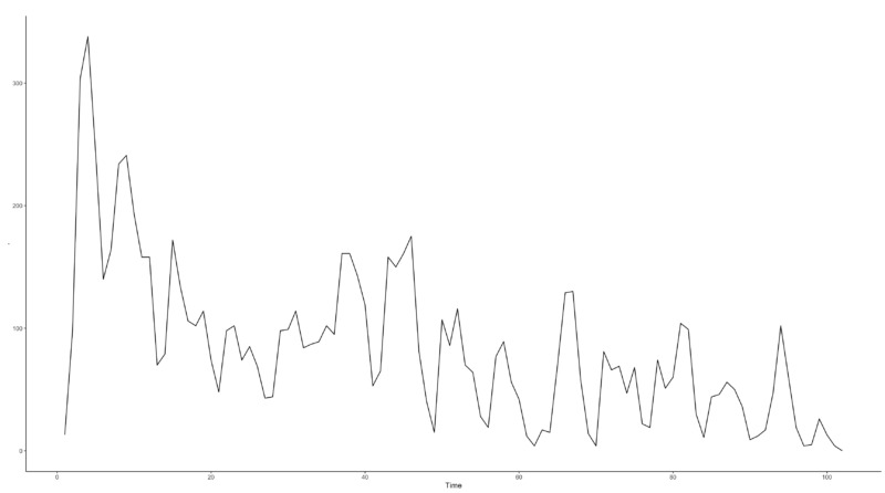
The raw data used in the study are the results of digital advertising run over a specific period in 2022. The independent variable is the marketing spend, and the dependent variable is the marketing conversion. Since the marketing conversion, such as 1, 2, etc. are count data with a low probability of occurrence, it can be inferred that modeling based on the Poisson model would be appropriate.

3.2 Data Preprocessing and Assumptions

The raw data were filtered with only performance data generated from marketing channels using marketing spend out of overall marketing performance. Generally, marketing performance obtained using marketing spend is referred to as “Paid Performance”, while performance gained without using marketing spend is classified as “Organic Performance”. There may be a correlation between organic and paid performance depending on factors such as the size of the service, brand recognition, and some exogenous factors. Moreover, each marketing channel has different influences, and they can affect each other, suggesting the application of a hierarchical model or a multivariate model. However, in this study, a univariate model was applied.

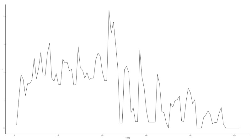
To verify the impact of measurement error, observation values were created by multiplying the actual marketing spend (true value) by the size of the measurement error. The reason for setting it multiplicatively is that the size of the measurement error is proportional to the marketing spend. At this point, considering that the observation value is inaccurate the more recent the data, the measurement error was set to increase exponentially the more it gets closer to the most recent value. As mentioned in the introduction, considering that media executing ads usually update data up to a week, measurement errors were applied only to the most recent 7 data points. The detailed process of the observed value is as follows.

\begin{gather}
e_{i} = \max(0, 1 + \eta_{i})\\
\eta_{i} \sim N(0, a(1+r)^{-\min(0, n-(i+7))})\\
spend^{*}_{i} = e_{i} * spend_{i}
\end{gather}

Where $e_{i}$ is the parameter representing the measurement error at time $i$. Since the ad spend cannot be negative, we set the Supremum to zero. The error is randomly determined by two parameters, $a$ and $r$, where $a$ is the scaling parameter and $r$ is the size of the error. We also accounted for the fact that the measurement error decreases exponentially over time.

As mentioned earlier, this measurement error is multiplicative, which can cause the variance of the residuals to increase non-linear. The magnitude of the measurement error is set to $[0.5, 1]$, which is not out of the domain, and simulated by Monte Carlo method ($n = 1,000$).

4. Data Modeling

Based on the aforementioned data, we define the independent and dependent variables for modeling. The dependent variable $count_{i}$ is the marketing conversion at time $i$, and the independent variable is the marketing spend at time $[i-7, i]$. The dependent variable is assumed to follow the following conditional Poisson distribution.

\begin{align}
count_{i} | spend_{i} \sim pois(\lambda)
\end{align}

The lag variable before the 7-day reflects the lag effect of users who have been influenced by an ad in the past, which causes marketing conversion to occur after a certain amount of time rather than on the same day. The optimal time may vary depending on the type of marketing action and industry, but we used 7-day performance as a universal.

First, let us apply a Distributed Lag Poisson Regression with true values that do not reflect measurement error and do not reflect autocorrelation effects. The equation and results are as follows.

\begin{align}
\log(\lambda_{t}) = \beta_{0} + \sum_{i=1}^{8}\beta_{i}Spend_{(t-i+1)}
\end{align}

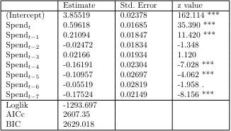
The results show that using the lag variable of 7 times is significant for model fit. To test the autocorrelation of the residuals, we derived ACF(Autocorrelation Function) and PACF(Partial Actucorrelation Function). In this case, we used Pearson residuals to consider the fit of the Poisson Regression Model.

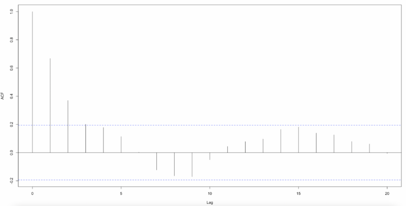
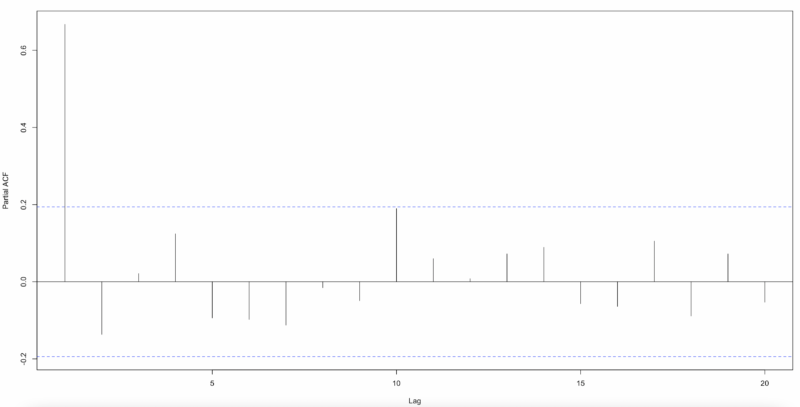
By the graph, there is autocorrelation in the residuals, so we need to add some time series parameters to reflect the model. The model equation with an autoregressive, mean average parameter that follows a Poisson distribution is as follows.

\begin{align}
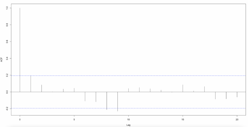
\log(\lambda_{t}) = \beta_{0} + \sum_{k=1}^{7}\beta_{k}\log(Y_{t-k} + 1) + \alpha_{7}\log(\lambda_{t-7}) + \sum_{i=1}^{8}\eta_{i}Spend_{(t-i+1)}
\end{align}

Where $\eta$ is the marketing spend used as an independent variable, $\beta$ is the intercept, and $\alpha$ is the unobserved conditional mean of the lagged variable of the dependent variable before 7 times, log-transformed into a log-linear model, which reflecting seasonality. The $\beta$ allows us to include effects that may affect the model other than the marketing spend used as a covariates, and the $\alpha$ is inserted to account for the effect of day of the week since the data is daily.

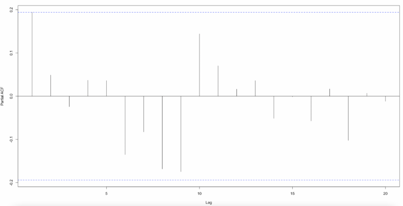
The results show that the lagged variables, $\alpha$ and $\beta$, are significant before 7 times. The quasi log-likelihood is also -874.725, which is a significant increase from before, and the AICc and BIC, which are indicators of model complexity, are also better for the Poisson Time Series.

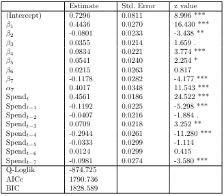
As shown below, when deriving ACF and PACF with Pearson residuals, we can see that autocorrelation is largely eliminated. Therefore, the results so far show that Poisson Time Series is better than Distributed Lag Poisson Regression.

And, we will simulate and include measurement error in our independent variable, marketing spend, and see how it affects our proposed models.

5. Results

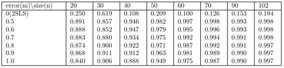
In this study, we evaluated the models on a number of criteria to understand the impact of measurement error and to determine which of the proposed models is superior. First, the “Prediction Accuracy” is an indicator of how well a model can actually predict future values, regardless of its fitting. The future values were set to 1 interval and measured by the Mean Absolute Error (MAE).

Since the characteristic of data follows time series structure, it is difficult to perform K-fold cross-validation or LOOCV(Leave One-Out Cross Validation) by arbitrarily dividing the data. Therefore, the MAE was derived by fitting the model with the initial $d$ data points, predicting 1 interval later, and then rolling the model to recursively repeat the same operation with one more data point. The MAE for the Poisson Time Series is as follows.

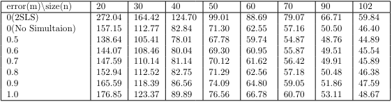
We can see that as the magnitude of the measurement error increases, the prediction accuracy decreases. However, at low levels of measurement error, we actually see lower MAE on average compared to performance evaluation on real data. This implies that instead of inserting bias into the model, the measurement error reduced the variance, which is more beneficial from an MAE perspective. The expression for MSE as a function of bias and variance is as follows.

\begin{align}
MSE = Bias^{2} + Var
\end{align}

If $Var$ decreases more than $Bias^{2}$ increases, we can understand that the model has developed from overfitting. MAE is the same, just a different metric. Therefore, with a reasonable measurement error size, the attenuation of the regression coefficient on the independent variable due to the measurement error can be understood as a kind of regularization effect.

However, for measurement errors above a certain size, the MAE is higher on average than the actual data. Therefore, if the measurement error is large, it is necessary to continuously update with new data by comparing with the data that is usually updated continuously, or to reduce the size of the measurement error by using the idea of repeated measures ANOVA(Analysis of Variance).

In some cases, you may decide that it is better to force additional regularization from the MAE perspective. In this case, it would be natural to use something like Ridge Regression, since the measurement error has been acting to dampen the coefficient effect in the same way as Ridge Regression.

Depending on the size of the data points, the influence of measurement error will decrease as the number of data points increases. This is because the error of measurement is only present for the last 7 data points, regardless of the size of the data points, hence the error of measurement gradually decreases as a percentage of the total data. Therefore, we can see that the impact of error of measurement is not significant in modeling situations where we have more than a certain number of data points.

However, in the case of digital advertising, there may be issues such as terminating ads within a short period of time if marketing performance is poor. Therefore, if you need to perform a hypothesis test with short-term data, you need to adjust the significance level to account for the effect of measurement error.

The 2SLS(2 Stage Least Squares) model, inserted in the table, will be proposed later to check the efficiency of the coefficients. Note that the 2SLS has a high MAE due to initial uncertainty, but as the data size increases, the MAE decreases rapidly compared to the original model.

Next, we need to determine the nature of the residuals in order to make more accurate and robust predictions. Therefore, we performed autocorrelation and heteroskedasticity tests on the residuals.

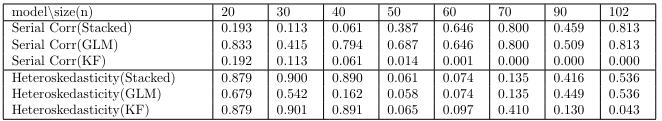
The following results is the autocorrelation test on the Pearson residuals. In this study, the Breusch-Godfrey test used in the regression model was performed on lag 7. In general, the Ljung-Box test is utilized, but the Ljung-Box test is the Wald test class, which has a high power under the strong exogeneity(Mean Independent) assumption between the residuals and independent variables\cite{Hayashi}. Therefore, the strong exogeneity assumption about Wald test are not appropriate for this study, which requires a test for measurement error and the case of few data points. On the other hand, the Breusch-Godfrey test has the advantage of being more robust than the Ljung-Box test, because it assumes more relaxed exogeneity(Same Row Uncorrelated) assumption under the Score test class.

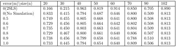
The test shows that the measurement error does not significantly affect the autocorrelation of the residuals.

Next, here are the results for the heteroskedasticity test. Although GLM-type models do not specifically assume homoskedasticity of the residuals, we still need to investigate the mean-variance relationship assumed in the modeling. To check this indirectly, we scaled the residuals as Pearson, and then performed a Breusch-Pagan test for heteroskedasticity.

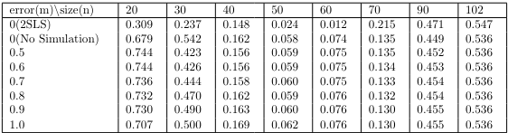
We can see that the measurement error does not significantly affect the assumed mean-variance relationship of the model. Consider the process of estimating the parameters in a GLM. The Information Matrix in (14) is weighted by the mean, whereas in Poisson Regression, the mean is same as variance, so it is weighted by the mean. Since it utilizes a weight matrix with a similar idea to GLS(Generalized Least Squares), it has the inherent effect of suppressing heterogeneity to a certain extent by giving lower weights to uncertain data.

On the other hand, we can see that the Breusch-Pagan test has a low p-value on some data points. If the significant level is higher than 0.05, the null hypothesis can be rejected. This is because there is a regime shift in the independent variable before and after $n = 47$, as shown in Fig. 1.

To test this, we performed a Quasi Likelihood Ratio Test(df = 9) between the saturated model, that considered the pattern change before and after the regime shift and the reduced model that did not consider it. The results are shown below.

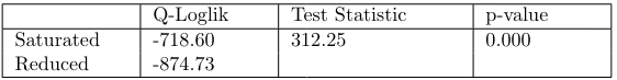
Since the test statistic exceeds the rejection bound and is significant at the significance level 0.05. It can be concluded that the interruption of ad delivery after the changepoint, or the lower marketing spend compared to before, may have affected the assumed mean-variance relationship. We do not consider this in our study, but it would be possible to account for regime shifts retrospectively or use a Negative Binomial based regression model to account for this.

Next, we test for efficiency of statistics. Although this study does not focus on the endogeneity of the coefficients, we use a 2SLS model as the specification for the efficiency test. The proposed instrumental variable is ad impressions. The instrumental variable should have two characteristics: first, it should be “Relevant”, which means that the correlation between the instrumental variable and the original variable is high. The variance of the regression coefficient estimated with the instrumental variable is higher than the variance of the model estimated with the original variable, and the higher the correlation, the more favorable it is to reduce the difference with the variance of the original variable(Highly Relevant). Since the ad publisher’s billing policy is “Cost per Impression”, the correlation between ad spend and impressions is significantly high.

On the other hand, “Validity” is most important for instrumental variables, which should be uncorrelated with the errors to eliminate endogeneity. In the digital advertising market, when a user is exposed to a display ad, the price of the ad is determined by two things: the number of “Impressions” and the “Strength of Competition” between real-time ad auction bidders. Since the effect of impressions has been removed from the residuals, it is unlikely that the remaining factor, the strength of competition among auction bidders, is correlated with the user being forced to see the ad. Furthermore, the orthogonality test below shows the difficulty in rejecting the null hypothesis of uncorrelated.

Therefore, we can see that it makes sense to use “Impressions” as an instrumental variable instead of marketing spend. Here are the proposed 2SLS equations.

\begin{gather}
\hat{Spend}_{t} = \gamma_{0} + \gamma_{1}Imp_{t}\\
\log(\lambda_{t}) = \beta_{0} + \sum_{k=1}^{7}\beta_{k}\log(Y_{t-k} + 1) + \alpha_{7}\log(\lambda_{t-7}) + \sum_{i=1}^{8}\eta_{i}\hat{Spend}_{t-i+1}
\end{gather}

It is known that if there is measurement error in the instrumental variable, the number of impressions, but the random measurement error in the instrumental variable does not affect the validity of the model.

We performed the Levene test and Durbin-Wu-Hausman test to see the equality of residual variances. Below is the result of the Levene test.

We can see that the measurement error does not significantly affect the variance of the residuals. Furthermore, 2SLS also shows that there is no significant difference in the variance of the residuals at the significance level 0.05. This means that the instrumental variable is highly correlated to the original variables.

The Durbin-Wu-Hausman test checks whether there is a difference in the estimated coefficients between the proposed model and the original model. If the null hypothesis is rejected, the measurement error has a significant effect and the variance of the residuals will be affected. The results of the test between the original model and the model with measurement error are shown in the table below. We can see that the presence of measurement error does not affect the efficiency of the model, except in a few cases.

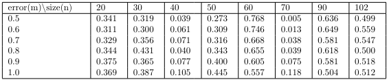
In addition, we check whether there is a difference in the coefficients between the proposed 2SLS and the original model. If the null hypothesis is rejected, it can be understood that there is an effect of omitted variables other than measurement error, which can affect the variance of the residuals. The results of the test are shown below.

When the data size is small, the model is not well specified and the 2SLS is more robust than the original model, but above a certain data size, there is no significant difference between the two models. In conclusion, the results of the above tests show that the proposed Poisson Time Series does not show significant effects of measurement error and unobserved variables. This is because, as mentioned earlier, the weight matrix-based parameter estimation method of AR, MA parameters, and GLM class model inherently suppresses some of these effects.

In addition to the GLM based Poisson Time Series, we also proposed a State Space Model based Poisson Kalman Filter. In the Poisson Kalman Filter, the inaccuracy of the observation equation due to measurement error is inherently corrected by the state equation, which has the advantage of being robust to measurement error problem.

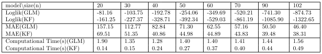
The table below shows the benchmark results between Poisson Time Series and Poisson Kalman Filter. You can see that the log-likelihood is always higher for the Poisson Time Series, but lower for the Poisson Kalman Filter in the MAE. This can be understood as the Poisson Time Series is more complex and overfitted, compared to the Poisson Kalman Filter.

However, after $n = 40$, the Poisson Time Series shows a rapid improvement in prediction accuracy. On the other hand, the Poisson Kalman Filter shows no significant improvement in prediction accuracy after a certain data point. This suggests that the model specification of the Poisson Time Series is appropriate beyond a certain data point.

We also compared the computational speed of the two models. We used “furrr” library in the R 4.3.1 environment, and ran 1,000 times each to derive the simulated value. In terms of computation time, the Poisson Time Series is about 1 second slower on average, but we do not believe this has a significant business impact unless you are in a situation where huge simulation is required.

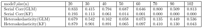
The following table below shows the test results for the residuals between the Poisson Time Series and the Poisson Kalman Filter. We can see the heterogeneity between the two models. In the case of the Poisson Kalman Filter, we can see that the evidence of initial autocorrelation and homoscedasticity is high, but the p-value decreases above a certain data size. This means that the Poisson Kalman Filter is not properly specified, when the data size increases.

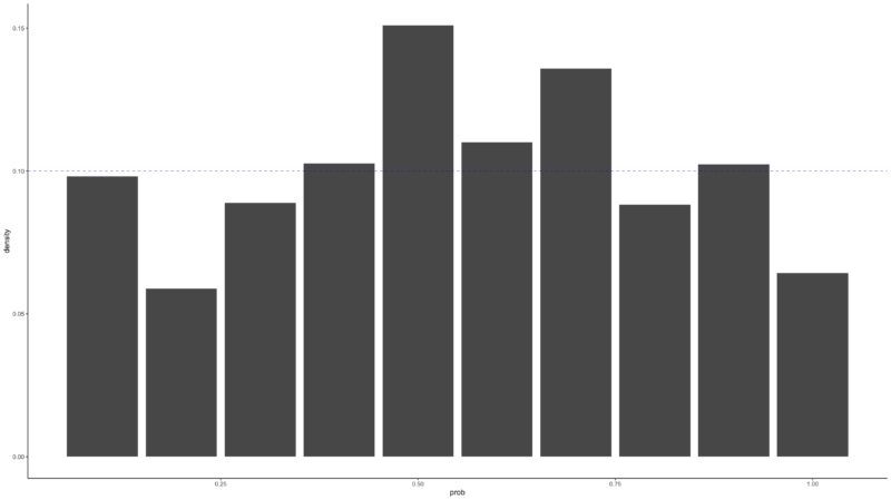
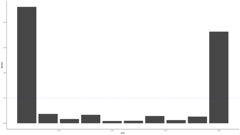
Finally, the PIT(Probability Integral Transform) allows us to empirically verify that the model is properly modeled by the mean-variance relationship. If the modeling was done properly, the histogram after the PIT should be close to a Uniform distribution. The farther it is from the Uniform distribution, the less it reflects the DGP of the original data. In the graph below, we can see that the Poisson Time Series shows values that do not deviate much from Uniform distribution, but the Poisson Kalman Filter results in values that are far from the distribution.

6. Ensemble Methods

So far, we have covered Poisson Time Series and the Poisson Kalman Filter. When the data size is small, the Poisson Kalman Filter is reasonable, but above a certain data size, the Poisson Time Series is reasonable. To reflect the heterogeneity of these two models, we want to derive the final model through model averaging. The optimization objective function is shown below.

\begin{gather}
p_{t+1} = argmin_{p}\sum_{i=1}^{t}w_{i}|y_{i} – (p \hat{y}_{i}^{(GLM)} + (1 – p) \hat{y}_{i}^{(KF)})|\\
s.t. \hspace{0.1cm} 0 \leq p \leq 1, \hspace{1cm} \forall w > 0
\end{gather}

The objective function is set in terms of minimizing the MAE, and different data points are weighted differently via the $w_{i}$ parameter. $w_{i}$ is the reciprocal of the variance at that point in time out of the total variance in precision, to reflect the fact that the more recent the data, the better the estimation and therefore the lower the variance. And the better the model, the lower the variance. The final weighted model prediction process is shown below.

\begin{align}
\hat{y}_{t+1} = p_{t+1}\hat{y}_{t+1}^{(GLM)} + (1 – p_{t+1})\hat{y}_{t+1}^{(KF)}
\end{align}

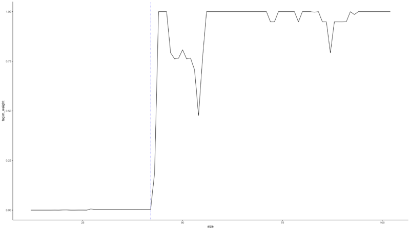
Below graph is the weights of the Poisson Time Series per data point derived from Stacking Methods. You can see that the weights are close to zero until $n = 42$, after which they increase significantly. In the middle, where the data becomes more volatile, such as the regime shift(blue vertical line), the weights are partially decreased.

The table below shows the results of the comparison between the final stacking model and the Poisson time series and Poisson Kalman Filter. First, we can see that the stacking model is superior in all times in the MAE, as it absorbs the advantages of both models, reflecting the Poisson Kalman Filter’s advantage when the data size is small, and the Poisson Time Series’ advantage above a certain data size. We can also see that the robustness test shows that the p-value of stacking model is laid between the p-values derived from both models.

7. Conclusion

We have shown the impact of measurement error on count data in the digital advertising domain. Even if the main purpose is not to build an analytical model but simply to build a model that makes better predictions, it is also important to check the measurement error in predictive modeling since the model may be underfitted by the measurement error, and the residuals may be heteroskedastic depending on the characteristic of the measurement error.

To this end, we introduced GLM based Poisson Time Series, and Poisson Kalman Filter, a class of Extended Kalman Filter, which can partially solve the measurement error problem. After applying these models to simulated data based on real data, the results of prediction accuracy and statistical tests were obtained.

In terms of prediction accuracy, we found that the magnitude of the coefficients is attenuated due to measurement error, causing a kind of regularization effect. For the data used in this study, we found that the smaller the measurement error, the better the prediction accuracy, while the larger the measurement error, the worse the prediction accuracy compared to the original data. We also found that the impact of the measurement error was relatively high when the data size was small, but as the data size increased, the impact of the measurement error became smaller. This is due to the nature of digital advertising data, where only recent data is subject to measurement error.

The test of residuals shows that there is no significant difference with and without measurement error. Therefore, the proposed models can partially avoid the problem of measurement error, which is advantageous in digital advertising data.

We also note that the two models are heterogeneous in terms of data size. When the data size is small and the impact of measurement error is relatively large, we found that the Poisson Kalman Filter, which additionally utilizes the state equation, is superior to the overspecified Poisson Time Series. On the other hand, as the data size increases, we found that the Poisson Time Series is gradually superior in terms of model specification accuracy. Finally, based on the heterogeneity of the two models, we proposed an ensemble class of stacking models that can combine their advantages. In the tests of prediction accuracy and residuals, the advantages of the two models were combined, and the final model showed better results than the single model.

On the other hand, while we assumed that the data follows a conditional Poisson distribution, some data points may be overdispersed due to volatility. This is evidenced by the presence of structural breaks in the retrospective analysis. If the data has overdispersion compared to the model, it may be more beneficial to assume a Negative Binomial distribution. Also, since the proposed data is a daily time series data, further research on increasing the frequency to hourly data could be considered. Finally, although we assumed a univariate model in this study, in the case of real-world digital advertising data, a user may be influenced by multiple advertising media simultaneously, so there may be correlation between media. Therefore, it would be good to consider a multivariate regression model such as SUR(Seemingly Unrelated Regression), which considers correlation between residuals, or GLMM(Generalized Linear Mixed Model), which considers the hierarchical structure of the data, in subsequent studies.

References

[1] Agresti, A. (2012). Categorical Data Analysis 3rd ed. Wiley.

[2] Biewen, E., Nolte, S. and Rosemann, M. (2008). Multiplicative Measurement Error and the Simulation Extrapolation Method. IAW Discussion Papers 39.

[3] Boyd, S. and Vandenberghe, L. (2004). Convex Optimization. Cambridge University Press.

[4] Czado, C., Gneiting, T. and Held, L. (2009). Predictive Model Assessment for Count Data. Biometrics 65, 1254-1261.

[5] Greene, W. H. (2020). Econometric Analysis 8th ed. Pearson.

[6] Greenshtein, E. and Ritov, Y. (2004). Persistence in high-dimensional linear predictor selection
and the virtue of overparametrization. Bernoulli 10(6), 971-988.

[7] Hayashi, F. (2000). Econometrics. Princeton University Press.

[8] Helske, J. (2016). Exponential Family State Space Models in R. arXiv preprint
arXiv:1612.01907v2.

[9] Hyndman, R. J., and Athanasopoulos, G. (2021). Forecasting: principles and practice 3rd ed.
OTexts. OTexts.com/fpp3.

[10] KOBACO. (2022). Broadcast Advertising Survey Report, 165-168.

[11] Liboschik, T., Fokianos, K. and Fried, R. (2017). An R Package for Analysis of Count Time Series
Following Generalized Linear Models. Journal of Statistical Software 82(5), 1-51.

[12] Liu, J. S. (2001). Monte Carlo Strategies in Scientific Computing. Springer.

[13] Montgomery, D. C., Peck, E. A. and. Vining, G. G. (2021). Introduction to Linear Regression
Analysis 6th ed. Wiley.

[14] Shmueli, G. (2010). To Explain or to Predict?. Statistical Science 25(3), 289-310.

[15] Shumway, R. H. and Stoffer, D. S. (2016). Time Series Analysis and Its Applications with R
Examples 4th ed. Springer.