Modeling Joint Distribution Of Monthly Energy Uses In Individual Urban Buildings For A Year

Jeonghun Song ^a, Hoyong Choi ^b,*

^a Swiss Institute of Artificial Intelligence, Chaltenbodenstrasse 26, 8834 Schindellegi, Schwyz, Switzerland

^b Graduate School of Innovation and Technology Management, College of Business, Korea Advanced Institute of Science and Technology, Daehak-ro, Yuseong-gu, Daejeon 34141, Republic of Korea

* Corresponding author, E-mail: [email protected]

1. Introduction

In 2021, the operation of buildings accounted for 30% of global final energy consumption and 27% of total energy sector emissions [1]. Energy saving in building sector is one of the most important activities to alleviate global warming and improve environmental sustainability. One of the key factors for energy saving in building sector is development of estimation methods for energy consumption in individual buildings. Such methods can provide information of building energy performance to decision makers related to energy policy making and energy infrastructure planning.

The methods for estimation of energy use in individual buildings can be separated into two categories – physical methods, and statistical methods [2, 3, 4]. Physical methods adopt detailed physical constraint-based models of building components and external conditions (e.g. detailed construction fabric, detailed shape, lightning and heating, ventilation and air conditioning system, indoor schedule, climate information), then estimate energy use in a target building by simulation tool. Statistical methods adopt regression models which contains energy use record of many individual buildings as the response variable, and features in building register (e.g. floor area, number of stories, category of construction fabric, construction date, etc.) as explanatory variables.

This study belongs to statistical methods, and there are several previous studies on statistical methods for estimation of annual energy use in individual buildings. Many of the studies provide estimation of annual energy use per floor area in the unit of kWh/m² year (often called as energy intensity), because the annual energy use of a target building can be estimated as the energy intensity multiplied with its floor area. Some studies have reported constant values of energy intensity of major building uses (e.g. office, retail, hospital, school, etc.) [5, 6, 7]. The other studies have provided linear regression models for estimation of annual energy consumption itself [8, 9] or energy intensity [4, 10, 11] as a function of building features.

This study focuses on ‘monthly’ energy use in individual buildings, which reflects seasonality of energy use. In general, electricity use in a building is relatively higher in summer due to cooling, while gas use in a building is relatively higher in winter due to heating. Such information of seasonality is helpful for scheduling of fuel supplies, maintenance operation of the utilities and negotiation of contracts between energy companies [12]. Aggregation of monthly energy use of buildings in an urban area enables planning of distributed energy infrastructure and estimation of total capacity of building-integrated energy sources [13]. Also, hourly energy demand pattern of a building, which is necessary for energy dispatch scheduling, can be estimated from the record of monthly energy use of the building [14, 15, 16].

There are a few previous studies on statistical estimation of monthly energy use in individual buildings, which have been feasible due to availability of open database of monthly energy use in many buildings [15]. The representative studies are as follows.

i) Catalina et al. [17] used linear regression to estimate heating demand in each month for heating period. The dataset has been generated by a dynamic simulation tool for building energy assessment. The explanatory variables are building characteristics (shape factor, transmittance coefficients, window to floor area ratio, etc.) and climate factors (outdoor temperature and global radiation).

ii) Kim et al. [18] used linear regression to estimate electricity use and gas use in each month for a year. The dataset has been obtained from Korean Management System for Building Energy Database. The explanatory variables are floor area, indicator variables for month, building use (neighborhood living or office), subdistrict, number of stories, fabric types of structure and roof.

iii) Xu et al. [19] used two-step k-means clustering to divide the dataset of monthly electricity use in buildings into 16 subsets, then fitted separate normal distribution to each subset. In the first step, the whole dataset has been divided into 4 subsets with respect to magnitude of electricity use. In the second step, each of the 4 subsets has been further divided into 4 subsets with respect to seasonal pattern of electricity use. The dataset has been obtained from smart meter dataset of six cities in Jiangsu province.

The common limitation of the previous studies on statistical estimation of monthly energy use in individual buildings is ignorance of correlation between energy uses in different months or different energy types. In practice, energy uses in different months are expected to be correlated. For example, a building which uses much more electricity in January compared to other buildings with similar size is expected to use much more electricity in February as well. In this sense, positive correlation between electricity uses in January and February is expected. Another example is that gas use for heating in a building depends on the amount of electricity used for electrified heating which is a substitute of gas heating. In this sense, negative correlation between electricity and gas uses in winter is expected.

Considering monthly electricity and gas uses for a year in a building as a 24-dimensional vector, the previous studies have reported information of mean vector and diagonal terms of covariance matrix of the 24-dimensional vector of monthly energy use in individual buildings. However, off-diagonal terms of covariance matrix have not been investigated yet. Information of full covariance matrix including off-diagonal terms enables construction of a ‘joint’ probability of the vector of monthly energy use in individual buildings. The joint probability model enables drawing vector samples of monthly energy uses in target buildings given their features, which would be helpful for energy planning for new urban towns with consideration of uncertainty in building energy demand. Also, the joint probability model can enhance data quality, by application to data imputation and prediction which can be done by consideration of correlation in data.

The objective of this study is to provide a statistical method for estimation of ‘joint’ probability distribution of ‘monthly’ energy uses for a year in individual urban building. Section 2 presents the dataset used in this study, subset and variable selection for regression, and data pre-processing. Section 3 presents estimation of moment conditions (mean vector and full covariance matrix) of the vector of monthly energy use in individual buildings, based on linear regression models. Section 4 presents the joint probability model and its applications. Section 5 concludes this study with a summary.

2. Data

2.1. Data description

The following two datasets have been merged and used – i) dataset of monthly electricity and gas use in individual non-residential buildings, provided by Korean Ministry of Land since late 2015; and ii) dataset of building register which includes features of building. Each row of the two datasets corresponds to a single building or multiple buildings corresponding to one address. Each column of the dataset of monthly electricity and gas use is record of electricity use or gas use for one month (in the unit of kWh). The columns of the dataset of building register include address, building use (e.g. office, living neighborhood, hospital, welfare, retail, school, etc), site area, sum of floor area in all stories, number of stories, structure of building and roof, approval date for use, etc.

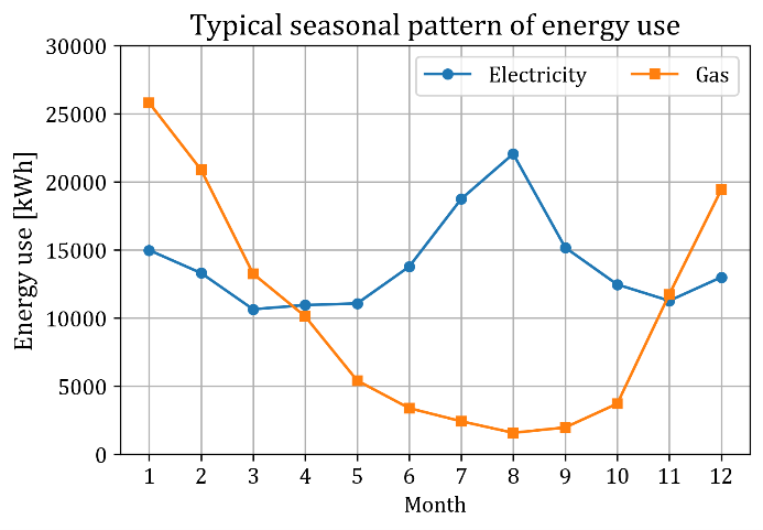
Figure 1 shows the typical seasonal pattern of monthly energy use in an exemplary building. The amount of electricity use is relatively higher in summer due to cooling, and relatively lower in spring and fall. The amount of electricity use in winter is usually similar to that in spring or fall. However, in some buildings, it may be as high as that in summer due to recently increasing electrification of heating. The amount of gas use in winter is relatively higher than that in other seasons due to heating. The amount of gas use in seasons other than winter varies much in different buildings depending on building use.

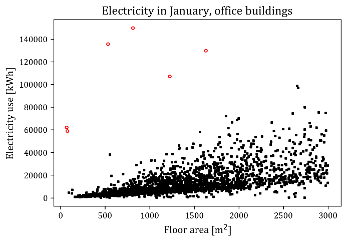
The dataset of monthly energy use in individual buildings has high variance. Figure 2 shows the electricity use in January 2021 in a subset of office buildings in Seoul, for varying floor area. Each data point in Figure 2 corresponds to one office building. The scatterplot presented a somewhat linear relationship, but instead of showing an intensive curve, the dots are more dispersed towards the end, especially dispersed for higher floor area. This spreading of the points implies two things – i) magnitude of energy use of buildings with similar size can be quite different from building to building, and ii) modern machine learning methods (like neural networks) with low bias but higher variance [20] are not appropriate for this dataset. Rather, traditional linear regression is appropriate for this dataset because linear regression is a method with high bias but lower variance.

2.2. Data setting

Among many features in the building register used in this study, the following features may be used to estimate the monthly energy use of individual buildings; floor area, building use, number of stories, approval year for use, category of building structure, and category of roof structure.

The features listed above can be explanatory variables for regression. For example, floor area of individual buildings can be an explanatory variable because the average energy use in individual buildings is expected to increase with increasing building size which is reflected by floor area.

Conversely, the dataset can be divided into subsets with respect to some of the features to make multiple regression models each for one subset. Division into subsets is necessary if the model coefficients are different from subset to subset. For example, the dataset can be divided with respect to building use because energy intensity, which is the coefficient of floor area, has been consistently found to be different for every building use in the previous studies on statistical estimation of energy use in buildings.

2.2.1. Subsets of the data

In this study, addition to building use, two additional criteria for subset division have been considered: interval of floor area, and use of gas. The two criteria for division has been selected due to the following reasons.

i) Interval of floor area: Floor area of individual buildings ranges in a very wide interval, from under 100 m² to over 100,000 m². In Seoul green building standard, the interval of floor area of a building has been divided into four subintervals – under 3,000 m², 3,000 m² to 10,000 m², 10,000 m² to 100,000 m², and over 100,000 m². Different standards of energy performance, management, and renewable energy penetration are applied to each subinterval. Thus, dividing the dataset with respect to the floor area intervals in the standard would make the result of this study practically available to users in energy policy field. Dividing into clusters obtained by k-means method as in [19] is not considered since it is hard to explain for domain purpose and the optimal classification boundaries can vary for different datasets. Taking log of floor area as in [18] is not considered because the important purpose of this research is to quantify covariance between monthly energy use in different months, not covariance between logged values of monthly energy use.

ii) Use of gas: Some buildings do not use gas, while others use gas. This difference has not been considered as a factor in the previous studies, but it is expected to affect average electricity use in winter because electricity and gas are substitutes for heating in winter. If a building does not use gas and meets its heating demand totally by electric heating, electricity use in winter is expected to be much higher than that in spring or fall. On the contrary, in a building which uses gas for meeting its heating demand, electricity use in winter is expected to be similar to that in spring or fall.

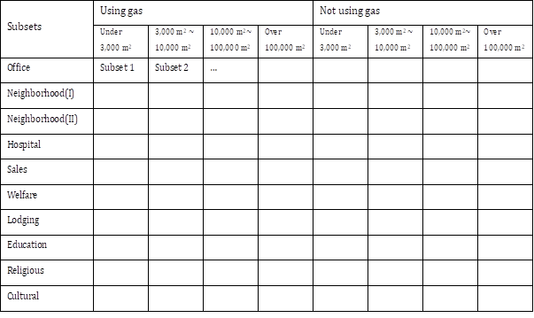
Table 1 shows the outline of subset division with respect to the three criteria. Subset division by interval floor area and use of gas will be justified by a statistical test explained in Section 2.2.3, based on linear regression with response variables and explanatory variables explained in Section 2.2.2.

2.2.2. Response and explanatory variables for regression

The response variables are electricity and gas use in individual months (for year 2021). For each subset of buildings which use gas, 24 linear regression models are fitted – 12 months multiplied with 2 energy types (electricity and gas). Thus, for a given set of explanatory variables, the mean of electricity or gas use in each month can be estimated separately.

The candidates for explanatory variables are as follows – floor area, number of stories, approval year for use of building (for example, a value 2000 means that the building has been used since year 2000), category of building structure, and category of roof structure. The category of building structure includes ferroconcrete, steel-concrete, steel-frame, brick, cement block, timber, etc. The category of roof structure includes ferroconcrete, slate, tile, etc. Among these candidates, variables to be used for fitting regression models should be determined.

A one-variable regression model including floor area as the only explanatory variable has been considered as the base model. Then, other regression models with additional explanatory variables and interaction terms between floor area and each of the additional explanatory variables have been compared with the base model, in terms of explanatory power (adjusted $R^2$). The interaction terms can reflect effects of the additional explanatory variables to the intercept and slope of the linear relationship between monthly energy use and floor. For demonstration, the subset of 2,326 office buildings using gas with floor area less than 3,000 m² has been selected.

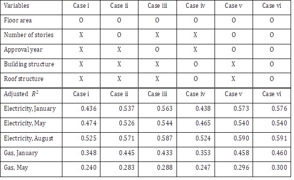
According to the demonstration, number of stories and approval year have been found to enhance explanatory power of the regression model. However, categories of building and roof structures have been found not to enhance explanatory power. Table 2 shows the values of adjusted $R^2$ for some selected months, corresponding to six cases – i) floor area only (base model); ii) floor area and number of stories; iii) floor area and approval year; iv) floor area and categories of building and roof structures; v) floor area, number of stories, and approval year; vi) all the explanatory variables mentioned above. Compared to the base model, the cases with number of stories or approval year showed greater adjusted $R^2$. However, the case with categories of structure but without number of stories and approval year showed little improvement in adjusted $R^2$.

Adding number of stories and approval year enhances explanatory power of the model because it makes the model reflect the following aspects – i) heating, ventilation, and air conditioning demand related to surface-volume ratio which is usually higher for tall buildings [21], ii) occupancy rate of the buildings due to business and commercial use which is usually higher for short buildings [18], iii) energy performance of electric appliances and insulation which is usually better for recently built buildings. Meanwhile, categories of building and roof structure could not enhance explanatory power in this study, because most of the buildings belong to one category of building structure and one roof structure. Depending on the building use, about 80~95% of buildings belong to ferroconcrete building and roof. Due to the imbalance of the categorical data, it is hard to estimate the average difference of energy use between different structures, resulting in little enhancement of explanatory power by adding category of structure to the regression models.

Consequently, three features have been adopted as the explanatory variables in this study – floor area, number of stories, approval year. Also, the interactions between floor area and number of stories, and between floor area and approval year have been included. Categories of structure have been excluded because they have little positive impact on explanatory power, and because the categorical variables make the model too complex due to many binary indicator variables. Although the number of stories is expected to increase with increasing floor area, multicollinearity problem is not expected. For example, the variation inflation factors of floor area, number of stories, and approval year in the model for electricity use in January without interaction terms are 1.447, 2.417, and 1.844, respectively, which are below 5.0 (which is the rule of thumb for potential multicollinearity).

2.2.3 Statistical test for subset division

To explain the regression-based statistical test, notations of the data are presented. Denote electricity and gas use in month m in building $i$ as $y_i^{elec,m}$ and $y_i^{gas,m}$, respectively. Then, 12-dimensional column vectors $y_i^{elec}=\left[y_i^{elec,1},\cdots,y_i^{elec,12}\right]^T$ and $y_i^{gas}=\left[y_i^{gas,1},\cdots,y_i^{gas,12}\right]^T$ are the record of monthly electricity and gas use for a year, respectively. For the regression model corresponding to electricity use in mth month, the data vector of response variable is $y^{elec,m}=\left[y_1^{elec,m},\cdots,y_N^{elec,m}\right]^T$ where N is the total number of data points. Also denote $x_i^{area}$, $x_i^{story}$ and $x_i^{year}$ as floor area, number of stories, and approval year of ith building, respectively. Then, the set of values of explanatory variables for $i$th data point is a six-dimensional vector $x_i=\left[1,x_i^{area},x_i^{story},x_i^{area}x_i^{story},x_i^{year},x_i^{area}x_i^{year}\right]^T$ (where 1 is added to estimate the intercept of the model), and the data matrix of explanatory variables is $X=\left[x_1,\cdots,x_N\right]^T$. The linear regression model for electricity use in mth month is presented as $y^{elec,m}=X\beta^{elec,m}+\epsilon^{elec,m}$, where $\beta^{elec,m}$ is the model coefficient vector and $\epsilon^{elec,m}=\left[\epsilon_1^{elec,m},\cdots,\epsilon_N^{elec,m}\right]^T$ is the error vector. The value of $\beta^{elec,m}$ can be estimated as ${\hat{\beta}}^{elec,m}=\left(X^TX\right)^{-1}X^Ty^{elec,m}$ by solving ordinary least squares problem, which aims to minimize the sum of squared errors $\left(\epsilon^{elec,m}\right)^T\epsilon^{elec,m}$. Using ${\hat{\beta}}^{elec,m}$, residual vector ${\hat{\epsilon}}^{elec,m}=y^{elec,m}-X{\hat{\beta}}^{elec,m}$ and residual sum of squares $SSR^{elec,m}=\left({\hat{\epsilon}}^{elec,m}\right)^T{\hat{\epsilon}}^{elec,m}$ can also be computed.

Suppose that partitioning $y^{elec,m}$ and $X$ into $\left[\left(y_A^{elec,m}\right)^T\ \ \left(y_B^{elec,m}\right)^T\right]^T$ and $\left[X_A^T\ \ X_B^T\right]^T$, respectively, is of interest. If partitioned, two separate regression models $y_A^{elec,m}=X_A\beta_A^{elec,m}+\epsilon_A^{elec,m}$ and $y_B^{elec,m}=X_B\beta_B^{elec,m}+\epsilon_B^{elec,m}$ can be constructed. If the true values of $\beta_A^{elec,m}$ and $\beta_B^{elec,m}$ are the same, the partitioning is meaningless since a single combined regression model $y^{elec,m}=X\beta^{elec,m}+\epsilon^{elec,m}$ would be sufficient to explain the whole data. On the contrary, the partitioning is necessary if the true values of $\beta_A^{elec,m}$ and $\beta_B^{elec,m}$ are different. Thus, the null hypothesis of the test is $\beta_A^{elec,m}=\beta_B^{elec,m}$ while the alternative hypothesis is $\beta_A^{elec,m}\neq\beta_B^{elec,m}$. The null hypothesis can be viewed as a set of equality restrictions to the model coefficients. From this view, $SSR_R^{elec,m}$ is defined as the residual sum of squares of the single combined model, the subscript $R$ means restricted. In the similar sense, $SSR_U^{elec,m}$ is defined as the sum of the two residual sum of squares of the two models each for one partition, where the subscript $U$ means unrestricted. Then, the test statistic (which approximately follows $F$ distribution under the null hypothesis) can be computed as in Equation 1 [22].

\begin{equation} \label{eq:F-test}
\frac{\left(SS\ R_R^{elec,m}-SSR_U^{elec,m}\right)/r}{SSR_U^{elec,m}/\left(N-k\right)}\sim\ F\left(r,N-k\right)
\end{equation}

where $r$ is the number of restrictions, and $k$ is the sum of the number of parameters in the separate regression models for each partition. The null hypothesis is rejected if the value of test statistic is over the critical value for a given significance level.

If a building dataset is partitioned based on use of gas, two partitions are made (using gas, not using gas). $r$ and $k$ are 6 and 12, respectively, since $\beta^{elec,m}$ is a six-dimensional vector. If a building dataset is partitioned based on floor area interval, four partitions are made (under 3,000 m², 3,000 m² to 10,000 m², 10,000 m² to 100,000 m², and over 100,000 m²). However, for the test in this study, only the first three partitions are considered for the test because the last partition contains only a few or even no buildings depending on the building use. For three partitions, $r$ and $k$ are 12 and 18, respectively.

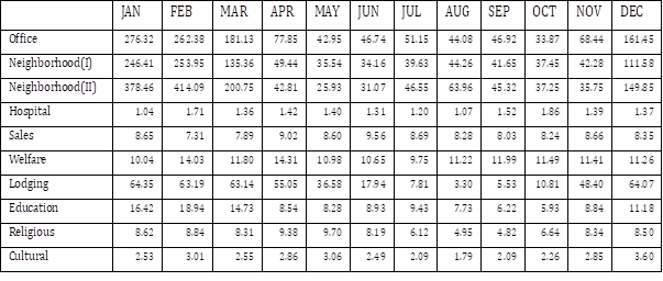
Table 3 shows that the null hypothesis of partitioning based on use of gas is rejected for most of the cases, which implies that it is necessary to partition the building dataset based on use of gas. Most of the values of test statistic computed for subsets, each corresponding to one of the buildings uses and floor area under 3,000 m², are over the critical value for 1% significance level $F_{0.01}\left(6,\infty\right)=2.803$. The values of test statistic are especially higher for winter, which supports the expected difference in magnitude of electricity use in winter depending on use of gas heating.

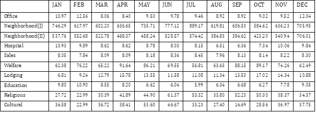
Table 4 shows that the null hypothesis of partitioning based on floor area interval is rejected for most of the cases, which implies that it is necessary to partition the building dataset based on floor area interval. Most of the values of test statistic computed for subsets, each corresponding to one of the buildings uses and buildings using gas, are over the critical value for 1% significance level $F_{0.01}\left(12,\infty\right)=2.187$.

It is noted that the statistical test has been done using the pre-processed dataset cleaned by the process explained in Section 2.3.

2.3. Data pre-processing

There is an issue of data quality of the raw dataset of monthly energy use in individual buildings because there are many abnormal data points which have missing or unrealistic values. In this study, abnormal data points are deleted from the dataset because the number of rows of the total dataset is large enough (order of 10⁴). The points with missing numbers, points with abnormal seasonal patterns, and points with abnormal magnitude of energy use have been deleted.

2.3.1. Data points with missing numbers

The detailed criteria of deletion are as follows:

i) Any of the 12 values of monthly energy use in the building is missing.

ii) Any of the 3 values of monthly gas use in the building in winter (January, February, and December) is missing or abnormally low if any of the values of gas use in other months is positive, because it is unusual that a building which uses gas during spring, summer or fall does not use gas or use only a small amount of gas in winter. It is noted that a data point with no record of gas use in all months is regarded as a building not using gas and preserved.

iii) Any of the values of monthly energy use is negative.

iv) Any of the values of explanatory variables is missing.

After applying the criteria to the dataset of buildings in Seoul for year 2021, 79,427 data points have been preserved.

2.3.2. Data points with abnormal seasonal patterns

Data points with abnormal seasonal patterns of energy use, which is far different from the exemplary pattern shown in Figure 1, have been deleted. Figure 3 shows examples of the abnormal seasonal patterns of monthly energy use in buildings. The cause of such abnormal patterns may be measurement error, or relatively rapid increasing or decreasing occupants. It is noted that the vertical axis in Figure 3 is the fraction of annual energy use for each month, to investigate only the shape of the seasonal patterns after control of the effect of building size on energy use.

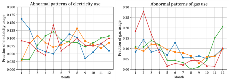
To apply the method for identification of data points with abnormal seasonal patterns, the dataset of monthly energy use in individual buildings has been transformed into a dataset of portion of annual energy use for each month. Dividing $y_i^{elec}$ with its absolute-value norm $\left|y_i^{elec}\right|_1$, the obtained vector ${\widetilde{y}}_i^{elec}=y_i^{elec}/\left|y_i^{elec}\right|_1$ represents fraction of annual electricity use for each month. ${\widetilde{y}}_i^{gas}=y_i^{gas}/\left|y_i^{gas}\right|_1$, which represents faction of annual gas use for each month, can be obtained in the same way. By aggregation of ${\widetilde{y}}_i^{elec}$ and ${\widetilde{y}}_i^{gas}$ of all buildings, new $N\times12$ data matrices ${\widetilde{Y}}^{elec}=\left[{\widetilde{y}}_1^{elec},\ \cdots\ {\widetilde{y}}_N^{elec}\right]^T$ and ${\widetilde{Y}}^{gas}=\left[{\widetilde{y}}_1^{gas},\ \cdots\ ,{\widetilde{y}}_N^{gas}\right]^T$, representing the transformed dataset, can be obtained.

A data point with abnormal seasonal pattern of electricity use can be considered as a point which is far from the cluster of points in the 12-dimensional vector space composed of row vectors in ${\widetilde{Y}}^{elec}$. A common approach to find such remote points in the vector space is to compute diagonal elements of the matrix ${\widetilde{Y}}^{elec}\left(\left({\widetilde{Y}}^{elec}\right)^T{\widetilde{Y}}^{elec}\right)^{-1}\left({\widetilde{Y}}^{elec}\right)^T$ (often called as hat matrix) [23]. ith diagonal element ${\widetilde{h}}_{ii}$ of the hat matrix can be written as in Equation 2.

\begin{equation} \label{eq:hat-matrix}
{\widetilde{h}}_{ii}=\left({\widetilde{y}}_i^{elec}\right)^T\left(\left({\widetilde{Y}}^{elec}\right)^T{\widetilde{Y}}^{elec}\right)^{-1}{\widetilde{y}}_i^{elec}
\end{equation}

A rule of thumb is to consider $i$th point as a remote point if ${\widetilde{h}}_{ii}$ is larger than $2k/N$ where $k$ is the dimension of the vector space (12 in this study). The points considered to be remote points following the rule of thumb were found to have abnormal seasonal patterns of electricity use as shown in Figure 3 and deleted from the dataset. The points which have abnormal seasonal patterns of gas use as shown in Figure 3 have been deleted in the same way. After deleting such points, the number of data points has been reduced from 79,427 to 68,135.

2.3.3. Data points with abnormal magnitude of energy use

Data points with unusually low or high energy use relative to other buildings with similar size may have a noticeable impact on the model coefficients, resulting in estimates of the coefficients far from its true value. Such points are often called the influential points, and the red hollow circles in Figure 2 are the points that are suspected to be influential points. The cause of such influential points may be measurement error, or unusual type of buildings (for example, energy use records of subway stations were found to be very high relative to the floor area of the station).

A common approach to find influential points is to compute Cook’s distance of every $i$th point, which is a measure of the squared distance between the estimated coefficient vector based on all points and the estimated coefficient vector obtained by deleting $i$th point [24]. Cook’s distance for $i$th point can be computed as in Equation 3.

\begin{equation} \label{eq:cook-distance}
D_i^{elec,m}=\frac{\left({\hat{\beta}}^{elec,m}-{\hat{\beta}}{-i}^{elec,m}\right)^TX^TX\left({\hat{\beta}}^{elec,m}-{\hat{\beta}}{-i}^{elec,m}\right)}{k\cdot M\ S\ R^{elec,m}}=\frac{{\hat{\epsilon}}i^{elec,m}h{ii}}{k\cdot M\ S\ R^{elec,m}\left(1-h_{ii}\right)^2}\end{equation}

where ${\hat{\beta}}{-i}^{elec,m}$ is the estimates of coefficients obtained by deleting ith point, k is number of coefficients (6 in this study), $MSR^{elec,m}=SSR^{elec,m}/\left(N-k\right)$ is the regression mean square of the model containing all points, and $h{ii}$ is $i$th diagonal element of $X\left(X^TX\right)^{-1}X^T$. It is not required to solve ordinary least squares problem $N+1$ times to obtain Cook’s distance of every point. By the term in the right side of equation 2, Cook’s distance of every point can be obtained by one computation of $X\left(X^TX\right)^{-1}X^T$ and solving ordinary least squares problem once.

Computation of Cook’s distance have been applied to each subset of Table 1 since computation of Cook’s distance requires regression models which are fitted for each of the subsets separately. For each subset,  is computed for every point. Then, the point which corresponds to the highest value of  is deleted because at least one of 12 monthly electricity uses in the corresponding building is abnormal in magnitude. This procedure is repeated until a pre-determined number of points are deleted from the dataset. If the subset is the set of buildings using gas, then buildings with abnormal monthly gas use in magnitude are also deleted, following the same procedure. In this study, the number of points to be deleted from each subset by this procedure has been pre-determined as two percent of the data points in the subset.

3. Estimation of moment conditions

3.1. Estimation based on linear regression models

To establish a joint probability model for monthly energy uses of a certain building given its features (floor area, number of stories, and approval year in this study) covariance between the error terms of two different regression models should be investigated. The linear regression model for electricity use in $m$th month can be written in pointwise form as Equation 4.

\begin{multline} \label{eq:linear-regression}
y_i^{elec,m}=\beta_0^{elec,m}+\beta_1^{elec,m}x_i^{area}+\beta_2^{elec,m}x_i^{story}+\beta_3^{elec,m}x_i^{area}x_i^{story}+\beta_4^{elec,m}x_i^{year}\\
+\beta_5^{elec,m}x_i^{area}x_i^{year}+\epsilon_i^{elec,m}
\end{multline}

Then, $\epsilon_i^{elec,1}$ and $\epsilon_i^{elec,2}$ are expected to be positively correlated because a building which uses more electricity in January compared to other buildings with similar size is expected to use more electricity in February compared to other buildings with similar size as well. Meanwhile, $\epsilon_i^{elec,1}$ and $\epsilon_i^{gas,1}$ are expected to be negatively correlated because electricity and gas are substitutes for heating in winter.

A common approach to estimate coefficients of many linear regression models simultaneously considering covariance between error terms of these regression models is Seemingly Unrelated Regression (SUR) [25]. SUR aggregates all of 24 regression models (12 for electricity, and 12 for gas) to make a combined regression model, as shown in matrix form in Equation 5.

\begin{equation} \label{eq:combined-regression}
\left[
\begin{matrix}
y^{elec,1}\\
y^{elec,2}\\
\vdots\\
y^{elec,12}\\
y^{gas,1} \\
\vdots\\
y^{gas,12}
\end{matrix}
\right]
=
\left[
\begin{matrix}
X^{elec,1} & 0 & \cdots & 0 & 0 & \cdots & 0 \\
0 & X^{elec,2} & \cdots & 0 & 0 & \cdots & 0 \\
\vdots & \vdots & \ddots & \vdots & \vdots & \ddots & \vdots \\
0 & 0 & \cdots & X^{elec,12} & 0 & \cdots & 0 \\
0 & 0 & \cdots & 0 & X^{gas,1} & \cdots & 0 \\
\vdots & \vdots & \ddots & \vdots & \vdots & \ddots & \vdots \\
0 & 0 & \cdots & 0 & 0 & \cdots & X^{gas,12}
\end{matrix}
\right]
\left[
\begin{matrix}
\beta^{elec,1}\\
\beta^{elec,2}\\
\vdots\\
\beta^{elec,12}\\
\beta^{gas,1}\\
\vdots\\
\beta^{gas,12}
\end{matrix}
\right]
+
\left[
\begin{matrix}
\epsilon^{elec,1}\\
\epsilon^{elec,2}\\
\vdots\\
\epsilon^{elec,12}\\
\epsilon^{gas,1}\\
\vdots\\
\epsilon^{gas,12}
\end{matrix}
\right]
\end{equation}

By solving generalized least squares problem for Equation 5, estimates of coefficients with consideration of covariance between error terms can be obtained. However, solving generalized least squares problem is more complicated than solving ordinary least squares problem because the exact structure of covariance is generally not known before solving.

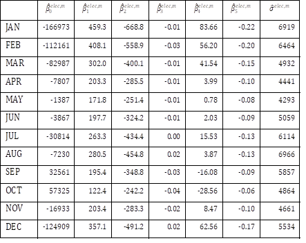
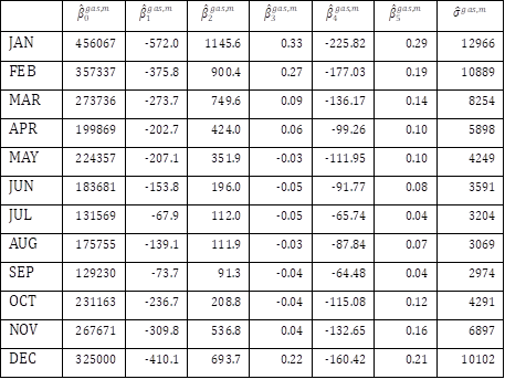
Fortunately, the generalized least squares estimators of SUR in this study are equivalent to the ordinary least squares estimators of each of the 24 regression models obtained separately, because all 24 models contain the same set of explanatory variables [25]. For example, Tables 5 and 6 shows the estimates of coefficients and standard error of the 24 models for the subset of 2,326 office buildings with floor area under 3,000 m² using gas, obtained by solving least squares of each of 24 regression models separately. Given the floor area and number of stories of a certain office building with floor area under 3,000 m² using gas, the mean vector of monthly energy use in the building can be determined by the estimates of coefficients. For other subsets, different estimates of coefficients would be obtained.

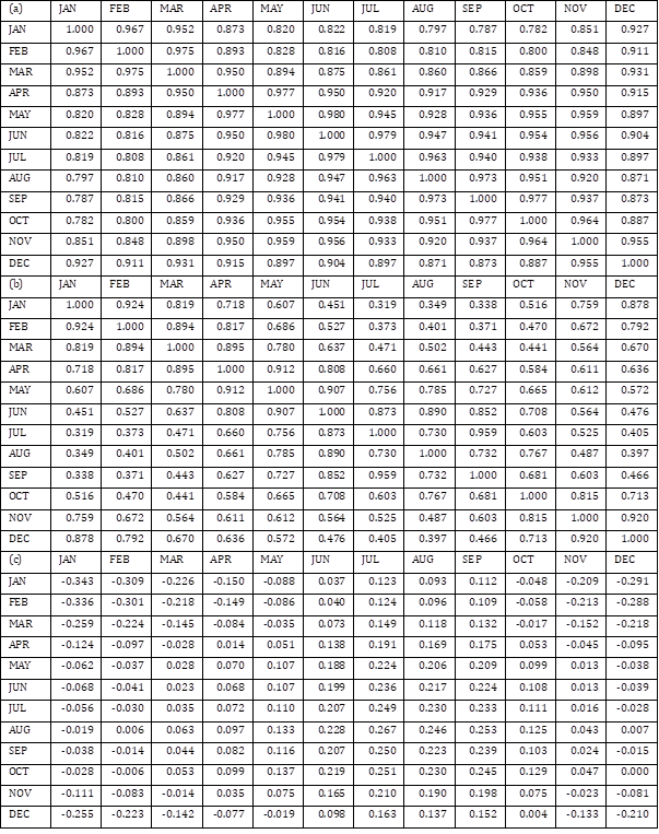
Covariance and correlation between error terms of different regression models can be estimated by computation of sample covariance matrix and sample correlation matrix of the residuals. Table 5 shows the sample correlation matrix of error terms of the 24 models for the subset of office buildings with floor area under 3,000 m² using gas. Table 7(a) shows that error terms corresponding to electricity use in different months are strongly positively correlated, even when the effects of size, height, and age of buildings have been controlled. This result supports the expectation on positive correlation between $\epsilon_i^{elec,1}$ and $\epsilon_i^{elec,2}$. Table 7(b) shows that error terms corresponding to gas use in adjacent different months are also strongly positively correlated. Table 7(c) shows that error terms corresponding to electricity use and gas use in winter are negatively correlated. This result supports the expectation on negative correlation between $\epsilon_i^{elec,1}$ and $\epsilon_i^{gas,1}$.

3.2. Issues of non-constant covariance (heteroskedasticity)

In Section 3.1, constant variance and covariance of error terms in each model has been assumed. If this assumption is violated, the estimation of covariance matrix based on as presented in Section 3.1 becomes invalid. Thus, it should be checked whether the variance and covariance are constant with all explanatory variables (homoscedastic) or they vary with at least one varying explanatory variable (heteroskedastic).

3.2.1. Existence of heteroskedasticity

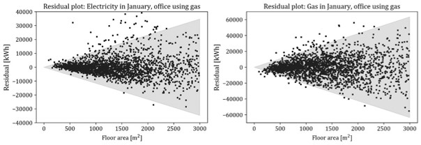
Figure 4, the residual plot, shows that variance of monthly energy use is not constant but increasing with increasing floor area. This heteroskedasticity has not been considered for obtaining sample covariance matrix in Section 3.1. Assuming homoskedasticity, the grey regions in Figure 4 represent the bands of $x_i^T{\hat{\beta}}^{elec,1}\pm2.58{\hat{\sigma}}^{elec,1}$ and $x_i^T{\hat{\beta}}^{gas,1}\pm2.58{\hat{\sigma}}^{gas,1}$, where ${\hat{\sigma}}^{elec,1}$ is the constant standard error of the regression model corresponding to electricity use in January. The band includes the region of large magnitude of residual with small floor area (depicted as dashed triangles), where there are few data points located in that region.

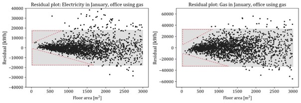
Thus, variance of energy use in small buildings will be overestimated so that unrealistically small or large amount of energy use can be sampled from the joint probability model based on assumption of constant variance. In contrast, variance of energy use in large buildings will be underestimated. Despite of such problem, issue of heteroskedasticity has not been considered in the previous studies on statistical estimation of building energy use. The structure of heteroskedasticity should be modeled to correct the estimation of covariance and to make a correct joint probability model.

3.2.2. Heteroskedasticity modeling

A common approach to estimate structure of heteroskedasticity in a linear regression model is to make an auxiliary regression model, where the response variable is the squared residual, and the explanatory variables are first and second order terms of explanatory variables which causes heteroskedasticity (floor area in this study) [26]. For the regression model corresponding to electricity use in $p$th month, the auxiliary regression model can be set up as in Equation 6.

\begin{equation} \label{eq:auxiliary-regression}
\left({\hat{\epsilon}}_i^{elec,p}\right)^2=\alpha_0^{elec,p}+\alpha_1^{elec,p}x_i^{area}+\alpha_2^{elec,p}\left(x_i^{area}\right)^2+v_i^{elec,p}
\end{equation}

where $v_i^{elec,p}$ is the error term of the auxiliary model. By estimation of the coefficients of the auxiliary model, variance can be estimated as a function of $x_i^{area}$, as in Equation 7.

\begin{equation} \label{eq:variance-auxiliary}
\left({\hat{\sigma}}^{elec,p}\right)^2=\ {\hat{\alpha}}_0^{elec,p}+\ {\hat{\alpha}}_1^{elec,p}x_i^{area}+\ {\hat{\alpha}}_2^{elec,p}\left(x_i^{area}\right)^2
\end{equation}

where $\left({\hat{\sigma}}^{elec,p}\right)^2$ denotes the estimate of error variance, and ${\hat{\alpha}}_0^{elec,p}$, ${\hat{\alpha}}_1^{elec,p}$, ${\hat{\alpha}}_2^{elec,p}$ denote the estimate of coefficients of the auxiliary model. $\left({\hat{\sigma}}^{gas,p}\right)^2$ as the function of floor area can also be obtained in the same way.

The explained approach can be extended to estimate the heteroskedasticity structure of covariance between error terms of two different regression models as a function of the explanatory variables [27]. For the two regression models corresponding to electricity uses in $p$th and $q$th months, the auxiliary regression model can be set up as in Equations 8 and 9.

\begin{equation} \label{eq:auxiliary-setup1}
{\hat{\epsilon}}_i^{elec,p}{\hat{\epsilon}}_i^{elec,q}=\alpha_0^{elec,\left(p,q\right)}+\alpha_1^{elec,\left(p,q\right)}x_i^{area}+\alpha_2^{elec,\left(p,q\right)}\left(x_i^{area}\right)^2+v_i^{elec,\left(p,q\right)}
\end{equation}

\begin{equation} \label{eq:auxiliary-setup2}
{\hat{\sigma}}_{\left(p,q\right)}^{e,e}=\ {\hat{\alpha}}_0^{elec,\left(p,q\right)}\ +\ {\hat{\alpha}}_1^{elec,\left(p,q\right)}\ x_i^{area}+\ {\hat{\alpha}}_2^{elec,\left(p,q\right)}\ \left(x_i^{area}\right)^2
\end{equation}

where ${\hat{\sigma}}{\left(p,p\right)}^{e,e}=\left({\hat{\sigma}}^{elec,p}\right)^2$ and $e$ in the superscript denotes electricity. ${\hat{\sigma}}{\left(p,q\right)}^{g,g}$ and ${\hat{\sigma}}_{\left(p,q\right)}^{e,g}$ can also be obtained in the same way (where $g$ in the superscript denotes gas).

However, estimate of covariance by Equation 9 may produce unrealistic value of covariance, such as negative variance and negative correlation between error terms of regression models corresponding to electricity use in January and February. For the subset of office buildings with floor area under 3,000 m² using gas, the variance of $\epsilon_i^{elec,1}$ and covariance between $\epsilon_i^{elec,1}$ and $\epsilon_i^{elec,2}$ have been estimated as ${\hat{\sigma}}{\left(1,1\right)}^{e,e}=-39278300+75969x_i^{area}-5.99\left(x_i^{area}\right)^2$ and ${\hat{\sigma}}{\left(1,2\right)}^{e,e}=-35607600+70291x_i^{area}-6.37\left(x_i^{area}\right)^2$, respectively. Both estimates become negative if $x_i^{area}$ is lower than about 500 m², which are practically positive but incorrectly estimated.

To prevent unrealistic estimation of covariance by change of sign, Equations 8 and 9 have been modified to contain only the second order term of floor area in the right side, as in Equations 10 and 11.

\begin{equation} \label{eq:modified-setup1}
{\hat{\epsilon}}i^{elec,p}{\hat{\epsilon}}_i^{elec,q}=\alpha{\left(p,q\right)}^{e,e}\left(x_i^{area}\right)^2+v_{\left(p,q\right),i}^{e,e}
\end{equation}

\begin{equation} \label{eq:modified-setup2}
{\hat{\sigma}}{\left(p,q\right)}^{e,e}=\ \ {\hat{\alpha}}{\left(p,q\right)}^{e,e}\ \left(x_i^{area}\right)^2
\end{equation}

The estimate of covariance matrix, constructed by aggregation of all estimates of covariance computed by Equation 11, is generally not positive semidefinite. However, a covariance matrix must be positive semidefinite by its properties. Thus, a positive semidefinite matrix nearest to the estimate of covariance matrix should be computed to be used as the covariance of the joint probability model of monthly energy uses.

The nearest positive semidefinite matrix can be obtained by eigen-decomposition. Denote the estimate of covariance matrix obtained by Equation 11 as $\hat{{\scriptstyle\sum}}$. $\hat{{\scriptstyle\sum}}$ is generally not positive semidefinite, but it is real-valued and symmetric. Thus, it can be decomposed as $\hat{{\scriptstyle\sum}}=VDV^T$ where $V$ is a square matrix containing eigenvectors of $\hat{{\scriptstyle\sum}}$ as its columns, and $D$ is a diagonal matrix containing eigenvalues of $\hat{{\scriptstyle\sum}}$ as its diagonal elements. Defining a new matrix $D_+$ which is obtained by replacing negative elements of $D$ with zeros, the nearest positive semidefinite matrix ${\hat{{\scriptstyle\sum}}}_+$ can be computed as ${\hat{{\scriptstyle\sum}}}_+=VD_+V^T$. Then, ${\hat{{\scriptstyle\sum}}}_+$ is used as the covariance matrix of the joint probability model for monthly energy uses. Table 8 shows the values of elements in ${\hat{{\scriptstyle\sum}}}_+$ for unit floor area, for the subset of office buildings with floor area under 3,000 m² using gas. The covariance matrix of the vector of monthly energy uses for a certain office building under 3,000 m² using gas can be obtained by multiplication of square of its floor area with the elements in Table 7. For other subsets, different estimates of covariance matrix would be obtained.

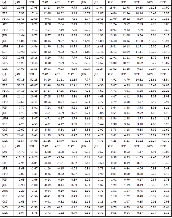
Figure 5 shows that the estimates of covariance from ${\hat{{\scriptstyle\sum}}}_+$ represents the heteroskedasticity of the data well. Adding a subscript $+$ which emphasizes that the covariance matrix is positive semidefinite, the modified bands $x_i^T{\hat{\beta}}^{elec,1}\pm2.58{\hat{\alpha}}_{\left(1,1\right)+}^{e,e}\ \left(x_i^{area}\right)^2$ and $x_i^T{\hat{\beta}}^{gas,1}\pm2.58{\hat{\alpha}}_{\left(1,1\right)+}^{g,g}\ \left(x_i^{area}\right)^2$ (depicted as grey areas) capture the increasing variance well while they do not contain regions where no data point is located.

4. Joint probability model

4.1. Multivariate normal distribution of monthly energy usage

A multivariate normal distribution for monthly electricity and gas uses for a year can be defined based on the mean vector and covariance matrix of monthly energy uses in a building obtained by the procedure presented in Section 3, conditional on the features of the building (floor area, number of stories, and approval year of the building), as Equation 12.

\begin{equation} \label{eq:multivariate-normal}
\left[
\begin{matrix}
y_i^{elec,1}\\
y_i^{elec,2}\\
\vdots\\
y_i^{elec,12}\\
y_i^{gas,1}\\
\vdots\\
y_i^{gas,12}
\end{matrix}
\right]
{\sim} MVN
\left(
\left[
\begin{matrix}
x_i^T{\hat{\beta}}^{elec,1}\\
x_i^T{\hat{\beta}}^{elec,2}\\
\vdots\\
x_i^T{\hat{\beta}}^{elec,12}\\
x_i^T{\hat{\beta}}^{gas,1}\\
\vdots\\
x_i^T{\hat{\beta}}^{gas,12}
\end{matrix}
\right]
,
\left[
\begin{matrix}
{\hat{\alpha}}_{\left(1,1\right)+}^{e,e} & {\hat{\alpha}}_{\left(1,2\right)+}^{e,e} & \cdots & {\hat{\alpha}}_{\left(1,12\right)+}^{e,e} & {\hat{\alpha}}_{\left(1,1\right)+}^{e,g} & \cdots & {\hat{\alpha}}_{\left(1,12\right)+}^{e,g}\\
{\hat{\alpha}}_{\left(2,1\right)+}^{e,e} & {\hat{\alpha}}_{\left(2,2\right)+}^{e,e} & \cdots & {\hat{\alpha}}_{\left(2,2\right)+}^{e,e} & {\hat{\alpha}}_{\left(2,1\right)+}^{e,g} & \cdots & {\hat{\alpha}}_{\left(2,12\right)+}^{e,g}\\
\vdots & \vdots & \ddots & \vdots & \vdots & \ddots & \vdots\\
{\hat{\alpha}}_{\left(12,1\right)+}^{e,e} & {\hat{\alpha}}_{\left(12,2\right)+}^{e,e} & \cdots & {\hat{\alpha}}_{\left(12,12\right)+}^{e,e} & {\hat{\alpha}}_{\left(12,1\right)+}^{e,g} & \cdots & {\hat{\alpha}}_{\left(12,12\right)+}^{e,g}\\
{\hat{\alpha}}_{\left(1,1\right)+}^{g,e} & {\hat{\alpha}}_{\left(1,2\right)+}^{g,e} & \cdots & {\hat{\alpha}}_{\left(1,12\right)+}^{g,e} & {\hat{\alpha}}_{\left(1,1\right)+}^{g,g} & \cdots & {\hat{\alpha}}_{\left(1,12\right)+}^{g,g}\\
\vdots & \vdots & \ddots & \vdots & \vdots & \ddots & \vdots\\
{\hat{\alpha}}_{\left(12,1\right)+}^{g,e} & {\hat{\alpha}}_{\left(12,2\right)+}^{g,e} & \cdots & {\hat{\alpha}}_{\left(12,12\right)+}^{g,e} & {\hat{\alpha}}_{\left(12,1\right)+}^{g,g} & \cdots & {\hat{\alpha}}_{\left(12,12\right)+}^{g,g}
\end{matrix}
\right]
\left(x_i^{area}\right)^2
\right)
\end{equation}

where MVN is the abbreviation of multivariate normal. The covariance matrix of the distribution contains $\left(x_i^{area}\right)^2$, meaning reflection of heteroskedasticity. There are two advantages of multivariate normal distribution – i) it is one of the simplest multivariate distributions for model construction, interpretation, maintenance, and sampling; and ii) it provides reasonable fit to near-symmetric data with high variance, which is the case of this study (Figure 6).

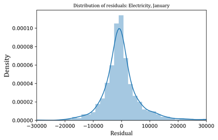
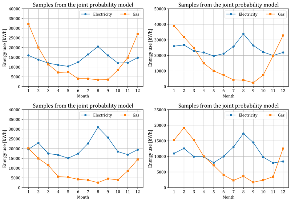
Figure 7 shows some samples of monthly energy use for one year drawn from the multivariate normal distribution fitted for the subset of office buildings using gas, conditional on floor area 1,500 m², seven stories, approved for use in 2000, which show reasonable seasonal patterns of energy use. The key to success in reflection of seasonality in monthly energy use is consideration of covariance between energy uses in different months or different energy types, which was not considered in previous studies. If the covariance is ignored, then samples drawn from the distribution which assumes independency of energy uses in different months or different energy types will show unrealistic seasonal patterns. Figure 8 shows some samples drawn from a different distribution with modified covariance matrix where its off-diagonal elements were replaced with zero. The samples show unrealistic seasonal patterns. Meanwhile, the magnitudes of energy use of the samples in Figure 7 are different to each other due to inevitable high variance nature of the data.

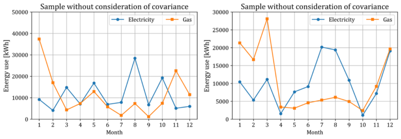
To obtain reasonable samples, a post-processing is required because a number of samples may show unrealistic seasonal patterns. Denote the monthly electricity use for a year in a sample drawn from the multivariate normal distribution as $y_0^{elec}$. Then, dividing it into its absolute value norm as ${\widetilde{y}}_0^{elec}=y_0^{elec}/\left|y_0^{elec}\right|_1$, the quantity $\left({\widetilde{y}}_0^{elec}\right)^T\left(\left({\widetilde{Y}}^{elec}\right)^T{\widetilde{Y}}^{elec}\right)^{-1}{\widetilde{y}}_0^{elec}$ can be computed (as similarly done in Section 2.3.2), where ${\widetilde{Y}}^{elec}$ multiplied with ${\widetilde{y}}_0^{elec}$ is the matrix composed of data preserved after pre-processing in Section 2.3.2. Samples with the quantity over a threshold ($2k/N$ in this study, but it can be adjusted by the user) are deleted. In a numerical experiment for the case of office building using gas with floor area 1,500 m² of floor area and seven stories, about 61% of initially drawn samples are preserved after the post-processing. On the contrary, when the post-processing is applied to the samples from the different distribution with ignorance of covariance between error terms for different months, none of the samples are preserved.

4.2. Application to data correction

In practice, some values in the record of monthly energy use in a building may be missing or incorrect. Figure 9 shows screenshots of some rows in the database of monthly energy use, which have missing or abnormally low values. If there is a method of filling the missing values or replacing unusual values with reasonable alternative values, it would help enhance data quality of the energy use record. However, models in previous studies with ignorance of covariance or simplified time-series models cannot be used for such task of data correction.

The joint probability model introduced in Section 4.1 can be used for data correction, based on the conditional multivariate normal distribution where the energy use in month with correct values in the record are assumed to be fixed. For a random vector variable $z=\left[z_1^T,\ z_2^T\right]^T$ following multivariate normal distribution where $z_2$ has been fixed to be $a$, the conditional multivariate normal distribution of $z_1$ can be expressed as Equation 13.

\begin{equation} \label{eq:conditional-mvn}
\left[\begin{matrix}
z_1\\
z_2
\end{matrix}\right]
{\sim}MVN
\left(\left[\begin{matrix}
\mu_1\\
\mu_2
\end{matrix}\right]
,
\left[\begin{matrix}
{\scriptstyle\sum}_{11} & {\scriptstyle\sum}_{12}\\
{\scriptstyle\sum}_{21} & {\scriptstyle\sum}_{22}
\end{matrix}\right]\right)
\Rightarrow\ P\left(z_1\middle| z_2=a\right)=MVN \left(\mu_1+ {\scriptstyle\sum}_{12} {\scriptstyle\sum}_{22}^{-1} \left(a-\mu_2 \right), {\scriptstyle\sum}_{11}- {\scriptstyle\sum}_{12} {\scriptstyle\sum}_{22}^{-1} {\scriptstyle\sum}_{21} \right)
\end{equation}

If $z$ is monthly electricity use for a year in a target building where electricity use values for some months $z_2$ are correct to be a but the values for the other months $z_1$ are missing or incorrect, the parameters $\mu_1$, $\mu_2$, ${\scriptstyle\sum}_{11}$, ${\scriptstyle\sum}_{12}$, ${\scriptstyle\sum}_{21}$, ${\scriptstyle\sum}_{22}$ become the electricity part of the mean and covariance the joint probability model in Equation 12. The mean of the conditional multivariate normal distribution $\mu_1+{\scriptstyle\sum}_{12}{\scriptstyle\sum}_{22}^{-1}\left(a-\mu_2\right)$ can be used as the alternative values for filling the missing values or replacing the incorrect values.

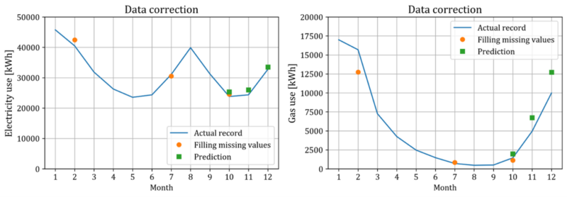
Figure 10 shows that the mean of the conditional multivariate normal distribution in Equation 13 produces reasonable alternative values. The curve denotes the actual recorded monthly energy use in the exemplary building with known floor area, number of stories and approval year. The circles denote the estimation of energy uses equal to the mean of the conditional multivariate normal distribution, assumed that the energy use record of the months corresponding to the circles (February, July, and October) are missing while record of the other months are available. The squares have the similar meaning as circles (assumed missing values in October, November, and December). The case of squares can be viewed as prediction of monthly energy use since the values of last three months are assumed to be missing and estimated given the energy use of preceding months. For electricity, the estimated values are quite close to the actual record. For gas, although the estimated values are a little deviated from the actual record due to the high variance of gas data, the new data generated by replacing the estimated values shows realistic seasonal pattern.

5. Summary

This study provides a statistical method to model the ‘joint’ probability distribution of ‘monthly’ electricity and gas uses for a year in individual urban buildings, conditional on the feature of the buildings. The process has been summarized as below:

i) Pre-process the database of monthly energy use and building features. Data points with missing values, or abnormal seasonal pattern of monthly energy use, or abnormal magnitude of energy use have been deleted. Points with abnormal seasonal pattern have been identified by a method which quantifies remoteness of each point from the cluster of the points applied to a transformed dataset. Points with abnormal magnitude of energy use have been identified by computation of Cook’s distance.

ii) For each subset of database (divided with respect to building use, floor area interval, use of gas), fit individual linear regression models. The response variable of each regression model is electricity or gas use in each month of buildings. In this study, the selected explanatory variables are floor area, number of stories, and approval year for use of buildings. Obtain the estimates of coefficients and residuals of the regression models.

iii) Establish auxiliary regression models to estimate the covariance of the errors as an increasing function of increasing floor area (in other words, estimate the structure of heteroskedasticity in the data). The response variable is multiplication of two residuals, each from regression models corresponding to the same or different months or energy types. The only explanatory variable is the square of floor area (no intercept). Transform the obtained estimate of covariance matrix into its nearest positive semidefinite matrix.

iv) Define a multivariate normal distribution conditional on the features of a building, where its mean vector is computed based on the estimates of coefficients obtained in ii) and its covariance matrix is computed based on the estimates of covariance matrix obtained in iii).

The joint probability model can be used to generate samples of monthly energy uses for a year in a target building, with realistic seasonal pattern and magnitude. Also, the joint probability model can be used to fill missing values or replace incorrect values of monthly energy use in a building with reasonable estimations, given that some correct values of monthly energy use are recorded in that building. The key to success of the provided model is the consideration of covariance between monthly energy uses, which exists even after controlling the effects of building size, height, and age.

References

[1] IEA (2022), Buildings, IEA, Paris https://www.iea.org/reports/buildings, License: CC BY 4.0

[2] Li, Z., Han, Y., & Xu, P. (2014). Methods for benchmarking building energy consumption against its past or intended performance: An overview. Applied Energy, 124, 325-334.

[3] Seyedzadeh, S., Rahimian, F. P., Glesk, I., & Roper, M. (2018). Machine learning for estimation of building energy consumption and performance: a review. Visualization in Engineering, 6(1), 1-20.

[4] Ciulla, G., & D’Amico, A. (2019). Building energy performance forecasting: A multiple linear regression approach. Applied Energy, 253, 113500.

[5] Turiel, I., Craig, P., Levine, M., McMahon, J., McCollister, G., Hesterberg, B., & Robinson, M. (1987). Estimation of energy intensity by end-use for commercial buildings. Energy, 12(6), 435-446.

[6] Pérez-Lombard, L., Ortiz, J., & Pout, C. (2008). A review on buildings energy consumption information. Energy and buildings, 40(3), 394-398.

[7] Zhong, X., Hu, M., Deetman, S., Rodrigues, J. F., Lin, H. X., Tukker, A., & Behrens, P. (2021). The evolution and future perspectives of energy intensity in the global building sector 1971–2060. Journal of Cleaner Production, 305, 127098.

[8] Olofsson, T., Andersson, S., & Sjögren, J. U. (2009). Building energy parameter investigations based on multivariate analysis. Energy and Buildings, 41(1), 71-80.

[9] Howard, B., Parshall, L., Thompson, J., Hammer, S., Dickinson, J., & Modi, V. (2012). Spatial distribution of urban building energy consumption by end use. Energy and Buildings, 45, 141-151.

[10] Andrews, C. J., & Krogmann, U. (2009). Technology diffusion and energy intensity in US commercial buildings. Energy Policy, 37(2), 541-553.

[11] Hsu, D. (2015). Identifying key variables and interactions in statistical models of building energy consumption using regularization. Energy, 83, 144-155.

[12] Apadula, F., Bassini, A., Elli, A., & Scapin, S. (2012). Relationships between meteorological variables and monthly electricity demand. Applied Energy, 98, 346-356.

[13] Song, J., & Song, S. J. (2020). A framework for analyzing city-wide impact of building-integrated renewable energy. Applied Energy, 276, 115489.

[14] Smith, A., Fumo, N., Luck, R., & Mago, P. J. (2011). Robustness of a methodology for estimating hourly energy consumption of buildings using monthly utility bills. Energy and Buildings, 43(4), 779-786.

[15] Pagliarini, G., & Rainieri, S. (2012). Restoration of the building hourly space heating and cooling loads from the monthly energy consumption. Energy and buildings, 49, 348-355.

[16] Lamagna, M., Nastasi, B., Groppi, D., Nezhad, M. M., & Garcia, D. A. (2020, December). Hourly energy profile determination technique from monthly energy bills. In Building Simulation (Vol. 13, No. 6, pp. 1235-1248). Tsinghua University Press.

[17] Catalina, T., Virgone, J., & Blanco, E. (2008). Development and validation of regression models to predict monthly heating demand for residential buildings. Energy and buildings, 40(10), 1825-1832.

[18] Kim, MK., Kim, BS., & Kim, JA. (2014). Development of a standard model for energy consumption in residential and commercial buildings in Seoul. City of Seoul, ISBN: 9791156212942 93530.

[19] Xu, J., Kang, X., Chen, Z., Yan, D., Guo, S., Jin, Y., … & Jia, R. (2021, February). Clustering-based probability distribution model for monthly residential building electricity consumption analysis. In Building Simulation (Vol. 14, No. 1, pp. 149-164). Tsinghua University Press.

[20] Hastie, T., Tibshirani, R., Friedman, J. H., & Friedman, J. H. (2009). The elements of statistical learning: data mining, inference, and prediction (Vol. 2, pp. 1-758). New York: springer.

[21] Araji, M. T. (2019, August). Surface-to-volume ratio: How building geometry impacts solar energy production and heat gain through envelopes. In IOP Conference Series: Earth and Environmental Science (Vol. 323, No. 1, p. 012034). IOP Publishing.

[22] Chow, G. C. (1960). Tests of equality between sets of coefficients in two linear regressions. Econometrica: Journal of the Econometric Society, 591-605.

[23] Hoaglin, D. C., & Welsch, R. E. (1978). The hat matrix in regression and ANOVA. The American Statistician, 32(1), 17-22.

[24] Cook, R. D. (1977). Detection of influential observation in linear regression. Technometrics, 19(1), 15-18.

[25] Davidson, R., & MacKinnon, J. G. (1993). Estimation and inference in econometrics (Vol. 63). New York: Oxford.

[26] Amemiya, T., & AMEMIYA, T. A. (1985). Advanced econometrics. Harvard university press.

[27] Mandy, D. M., & Martins-Filho, C. (1993). Seemingly unrelated regressions under additive heteroscedasticity: Theory and share equation applications. Journal of Econometrics, 58(3), 315-346.