Fiscal Games in Overlapping Jurisdictions

Jay Hyoung-Keun Kwon^*

^* Swiss Institute of Artificial Intelligence, Chaltenbodenstrasse 26, 8834 Schindellegi, Schwyz, Switzerland

I. Introduction

Recent developments in the urban landscape—such as sub-urbanization, counter-urbanization, and re-urbanization—have given rise to complicated scenarios where administrative jurisdictions are newly formed and intersect with existing ones. This presents unique challenges to traditional models of tax competition. This paper examines the economic implications of such overlapping jurisdictions, particularly focusing on their impact on tax policy.

Overlapping jurisdictions are characterized by multiple local governments exercising different levels of authority over the same geographic area. These arrangements often merge as responses to address urban sprawl or provide specialized services tailored to local needs. However, they also create a intricate network of fiscal relationships that can lead to inefficiencies in resource allocation and public service delivery.

For instance, local governments in the U.S., including counties, cities, towns, and special districts, have varying degrees of taxing powers. Residents in certain areas might be subject to property taxes levied by their town, county, school district, and special districts (such as fire or library districts), all operating within the same geographic space. This multi-layered governance structure not only affects residents’ tax burdens but also influences local governments’ decision-making processes regarding tax rates and public service provision. The resulting fiscal landscape provides a rich setting for examining the dynamics of tax competition and cooperation among overlapping jurisdictions.

Traditional models of tax competition, such as Wilson [4] and Zodrow and Mieszkowski [5], typically assume clear demarcations between competing jurisdictions. However, these models do not adequately capture the dynamics of overlapping administrative divisions. In such settings, local governments must navigate not only horizontal competition with neighboring jurisdictions but also a form of vertical competition within the same geographic space.

This paper aims to extend the literature on tax competition by developing a theoretical framework that accounts for the unique characteristics of overlapping jurisdictions. Specifically, we address the following research questions:

1. How do overlapping administrative divisions affect the strategic tax-setting behavior of local governments?
2. What are the implications of such overlapping structures for the provision of public goods and services?
3. How does the presence of overlapping jurisdictions influence the welfare outcomes predicted by traditional tax competition models?

To address these questions, we develop a game-theoretic model that incorporates multiple layers of local government operating within the same geographic space. This approach allows us to analyze the strategic interactions between overlapping jurisdictions and derive insights into the resulting equilibrium tax rates and levels of public good provision.

Our analysis contributes to the existing literature in several ways. First, it provides a formal framework for understanding tax competition in the context of overlapping jurisdictions, which is increasingly relevant in modern urban governance. Second, it offers insights into the potential inefficiencies that arise from such administrative structures and suggests possible policy interventions to mitigate these issues. Finally, it extends the theoretical foundations of fiscal federalism to account for more complex governance arrangements.

Our study addresses the current realities of fiscal federalism in developed economies as well as provides valuable insights for countries where local governments are yet to achieve significant fiscal autonomy. The lessons drawn from this analysis can inform policy discussions on decentralization, local governance structures, and intergovernmental fiscal relations in various contexts.

The remainder of this paper is organized as follows: Section II reviews the relevant literature on tax competition and fiscal federalism. Section III presents our theoretical model and derives key equilibrium results. Section IV discusses the implications of our findings for public policy and urban governance. Section V concludes and suggests directions for future research.

II. Literature Review

Tax competition has been one of the central themes in public economics. Tiebout [1]’s seminal work on local public goods laid the foundation for this field, proposing a model of “voting with feet” where residents moving to jurisdictions offering their preferred combination of taxes and public services. Oates [2] further developed these ideas and presented the decentralization theorem which posits that, under certain conditions, decentralized provision of public goods is welfare-maximizing.

Works of Wilson [4] and Zodrow and Mieszkowski [5] developed the basic tax competition model, where jurisdictions compete for a mobile capital tax base. This model predicts inefficiently low tax rates and underprovision of public goods, which is often referred to as the “race to the bottom.” Wildasin [6] further demonstrated that the Nash equilibrium in tax rates is generally inefficient by incorporating strategic interactions between jurisdictions.

Researchers began to consider more diverse institutional settings. Keen and Kotsogiannis [11] analyzed the interaction between vertical tax competition (between different levels of government) and horizontal tax competition (between governments at the same level). Their work demonstrated that in federal systems, the tax rates can be high or low depending on the relative strength of vertical and horizontal tax externalities, contrary to the “race to the bottom” prediction of earlier models.

Itaya, Okamura, and Yamaguchi [12] examined tax coordination in a repeated game setting with asymmetric regions. They find that the sustainability of tax coordination depends on the degree of asymmetry between regions and the type of coordination–partial or full. While asymmetries can complicate coordination efforts, the repeated nature of interactions can facilitate cooperation under certain conditions. Their work demonstrates that full tax coordination can be sustained for a wider range of parameters compared to partial coordination.

Building on this, Ogawa and Wang [14] incorporated fiscal equalization into the framework of asymmetric tax competition in a repeated game context. Their findings reveal that fiscal equalization can influence the sustainability of tax coordination, sometimes making it more difficult to maintain. The impact of equalization schemes on tax coordination is contingent on the degree of regional asymmetry and the specific parameters of the equalization policy.

The case of overlapping jurisdictions represents a frontier in tax competition research. While not extensively studied, some works have begun to address such cases. Hochman, Pines, and Thisse [9] developed a model of metropolitan governance with overlapping jurisdictions, showing how this can lead to inefficiencies in public good provision. Esteller-Mor´e and Sol´e-Oll´e [10] analyzed tax mimicking in a setting with overlapping tax bases, finding evidence of both horizontal and vertical interactions.

Game-theoretic approaches have been instrumental in advancing our understanding of tax competition dynamics. Wildasin [6] pioneered the use of game theory in tax competition, modeling jurisdictions as strategic players in a non-cooperative game. This approach demonstrated that the Nash equilibrium in tax rates is generally inefficient, providing a formal basis for the “race to the bottom” hypothesis. The work of Itaya, Okamura, and Yamaguchi [12] and Ogawa and Wang [14] further extended this game-theoretic approach to repeated games, offering insights into the possibilities for tax coordination over time.

While these game-theoretic approaches have significantly advanced our understanding of tax competition, they have largely failed to address the complexities of fully overlapping jurisdictions. Most models assume clear boundaries between competing jurisdictions, leaving a gap in our understanding of scenarios where multiple levels of government have taxing authority over the same geographic area.

The welfare implications of tax competition have been a subject of ongoing debate. While the “race to the bottom” hypothesis suggests negative welfare consequences, some scholars have argued for potential benefits. Brennan and Buchanan [3] proposed that tax competition could serve as a check on the excessive growth of government, a view that has found some support in subsequent empirical work (e.g., [13]).

Policy responses to tax competition have also been extensively studied. Proposals range from tax harmonization [7] to the implementation of corrective subsidies [8]. The effectiveness of these measures, particularly in complex settings with overlapping jurisdictions, remains an active area of research.

While the literature on tax competition has made significant strides in understanding the dynamics of fiscal interactions between jurisdictions, several areas warrant further investigation. The case of fully overlapping jurisdictions, in particular, presents a rich opportunity for both theoretical modeling and empirical analysis. This study aims to fill in this gap by accounting for overlapping jurisdictions in traditional game-theoretic models of tax competition.

III. Model

This study extends the tax competition models of Itaya, Okamura, and Yamaguchi [12] and Ogawa and Wang [14] by introducing an overlapping jurisdiction. Our approach is grounded in the Solow growth model, which provides a robust framework for analyzing long-term economic growth and capital accumulation. The Solow model’s emphasis on capital accumulation and technological progress makes it suitable for our analysis of tax competition, as these factors influence jurisdictions’ tax bases and policy decisions.

The Solow model’s assumptions of diminishing returns to capital and constant returns to scale align well with our focus on regional differences in capital endowments and production technologies. Moreover, its simplicity allows for tractable extensions to multi-jurisdiction settings.

A. Setup

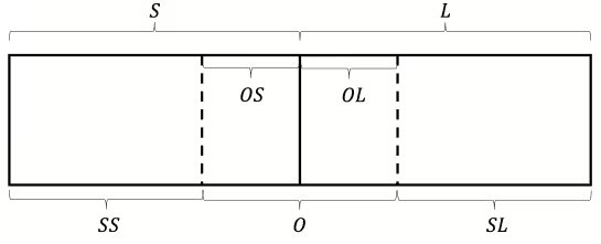
We consider a country divided into three regions: two asymmetric regions, $S$ and $L$, and an overlapping region, $O$, which equally overlaps with $S$ and $L$. All regions have independent authority to impose capital taxes. This setup allows us to examine the interactions between horizontal tax competition (between $S$ and $L$) and the unique dynamics introduced by the overlapping jurisdiction $O$. Let us further denote that the regions of $S$ and $L$ that do not overlap with $O$ are $SS$(Sub-$S$) and $SL$(Sub-$L$), respectively, while those that overlap with $O$ are $OS$ and $OL$ (see Figure 1).

Here, we make the following key assumptions:

1. Population: Population is evenly spread across the country. Hence, regions $S$ and $L$ have equal populations. Furthermore, regions $SS$, $SL$, and $O$ have equal populations. This assumption, while strong, allows us to isolate the effects of capital endowment and technology differences.
2. Labor Supply and Individual Preferences: Residents inelastically supply one unit of labor to firms in their region and have identical preferences. Furthermore, they strive to maximize their utilities given their budget constraints. While this assumption simplifies labor market dynamics, it is reasonable in the short to medium term, especially in areas with limited inter-regional mobility.
3. Production: Firms in each region produce homogeneous consumer goods and maximize their profits. This assumption allows us to focus on capital allocation without the complications of product differentiation.
4. Capital Mobility: Capital is perfectly mobile across regions, reflecting the ease of capital movement in economies, especially within a single country.
5. Asymmetric Endowments and Technology: Regions $S$ and $L$ differ in capital endowments and production technologies. This assumption captures real-world regional disparities and is crucial for generating meaningful tax competition dynamics.
6. Public Goods Provision: Regions $S$ and $L$ provide generic public goods $G$, while region $O$ provides specific public goods $H$ to the extent that maximizes their representative resident’s utilities. This reflects the often-observed division of responsibilities between different levels of government.

These assumptions, while simplifying the real world, allow us to focus on the core mechanisms of tax competition in overlapping jurisdictions. They provide a tractable framework for analyzing the strategic interactions between jurisdictions while capturing key elements of real-world complexity.

B. Production and Capital Allocation

Let $\bar{k}_i$ be the capital endowment per capita for regions $i$ and $\bar{k}$ be the capital endowments per capita of the national economy. For regions $S, L$ and $O$, it can be expressed as follows:

\begin{align}
\bar{k}_{s} \equiv \bar{k} – \varepsilon,\ \ \ \ \ \ \ \ \ \ \bar{k}_{L} \equiv \bar{k} + \varepsilon,\ \ \ \ \ \ \ \ \ \ \bar{k}_O = \bar{k} \equiv \frac{\bar{k}_{s} + \bar{k}_{L}}{2}
\end{align}

where $\varepsilon \in \left( 0,\ \bar{k} \right\rbrack$ represents asymmetric endowments between regions $S$ and $L$. $\bar{k}_O = \bar{k}$ follows from the assumption that the population is evenly dispersed across the country.

Let $L_i$ and $K_i$ be the labor and capital inputs for production in region $i$. It can be easily inferred that

\begin{align}
    l\equiv L_S = L_L , \ \ \ \ \ \ \ \ \ \ \frac{2}{3}l \equiv L_{SS} = L_{SL} = L_{O}.
\end{align}

Furthermore, we denote

\begin{align}
    K_{SS} \equiv \alpha_S K_S, \ \ \ \ \ \ \ \ \ \  K_{SL} \equiv \alpha_L K_L
\end{align}

for $0 < \alpha_S, \alpha_L < 1$.

With the key variables defined, the production function for each region $i$ is given by:

\begin{align}
    F_i(L_i, K_i) = A_i L_i + B_i K_i – \frac{K_i^2}{L_i}
\end{align}

where $A_i$ and $B_i > 2K_i / L_i$ represent labor and capital productivity coefficients, respectively. Although regions $S$ and $L$ differ in capital production technology, there is no difference in labor production technology, so $A_{L} = A_{S}$ while $B_{L} \neq \ B_{S}$. Note that this function exhibits constant returns to scale and diminishing returns to capital. Furthermore, we assume that sub-regions without overlaps ($SL$ and $SS$) have equivalent technology coefficients with their super-regions ($L$ and $S$). The technology parameter of the overlapping region is a weighted average of $B_S$ and $B_L$, where the weights are the proportion of capital invested from $S$ and $L$.

As mentioned above, capital allocation across regions is determined by profit-maximizing firms and the free movement of capital. Let $\tau_i$ be the effective tax rate for region $i$. Then, we can infer that the real wage rate $w_i$ and real interest rates $r_i$ are:

\begin{equation}
\begin{aligned}
    w_i &= A_i + \left(\frac{K_i}{L_i}\right)^2 \\
    r_i &= B_i – 2K_i/L_i – \tau_i – t_i
\end{aligned}
\end{equation}

where $t_i = (1-\alpha_i)\tau_O$ for $i \in \{S, L\}$, $0$ for $i\in \{SS, SL\}$, $\tau_S$ for $i = OS$, and $\tau_L$ for $i = OL$.

The capital market equilibrium for the national economy is reached when the sum of capital demands is equal to the exogenously fixed total capital endowment: $K_S + K_L = 2l\bar{k}$. In equilibrium, the interest rates and capital demanded in each region are as follows:
\begin{equation}
\begin{aligned}
    &r^* = \frac{1}{2}\big(\left(B_S + B_L \right) – \left(\tau_S + \tau_L + (2-\alpha_S-\alpha_L)\tau_O\right)\big) – 2\bar{k} \\
    &K_S^* = lk_S^* = l\bigg(\bar{k} + \frac{1}{4}\big( (\tau_L – \tau_S – (\alpha_L – \alpha_S)\tau_O ) – (B_L – B_S)\big) \bigg) \\
    &K_L^* = lk_L^* = l\bigg(\bar{k} + \frac{1}{4}\big( (\tau_S – \tau_L + (\alpha_L – \alpha_S)\tau_O ) + (B_L – B_S)\big) \bigg) \\
    &K_{SS}^* = \frac{2}{3}lk_{SS}^* = \frac{2l}{3}\bigg(\bar{k} + \frac{1}{4}\big( (\tau_L – \tau_S + (2 – \alpha_L – \alpha_S)\tau_O ) – (B_L – B_S)\big) \bigg) \\
    &K_{SL}^* = \frac{2}{3}lk_{SL}^* =\frac{2l}{3}\bigg(\bar{k} + \frac{1}{4}\big( (\tau_S – \tau_L + (2 – \alpha_L – \alpha_S)\tau_O ) + (B_L – B_S)\big) \bigg) \\
    &K_O^* = \frac{2}{3}lk_O^* = \frac{2l}{3}\left(\bar{k} – \frac{1}{2}(2-\alpha_S-\alpha_L)\tau_O\right)
\end{aligned}
\end{equation}
We denote $B_L – B_S = \theta$, henceforth.

C. Government Objectives and Tax Rates

Given that individuals in the country have identical preferences and inelastically supply one unit of labor to the regional firms, we can infer that all inhabitants receive a common return on capital of $r^*$ eventually, and they use all income to consume private good $c_i$. Hence, the budget constraint for an individual residing in region $i \in \{S, L, O\}$ and the sum of individuals in region $i$ will be

\begin{equation}
\begin{aligned}
    c_i &=  w_i^* + r^*\bar{k}_i   \\
    C_i &= \begin{cases}
        l(w^*_i + r^*\bar{k}_i) & \text{ for } i \in \{S, L\}\\
        \dfrac{2l}{3}(w^*_i + r^*\bar{k}) & \text{ for } i = O
    \end{cases}
\end{aligned}
\end{equation}

In addition, we have assumed that the overlapping district is a special district providing a special public good–for example education or health–that the other two districts do not provide. $S$ and $L$ provide their local public goods $G_i$. Then the total public goods provided in region $i$ can be expressed as:

\begin{equation}
\begin{aligned}
    G_i &= \begin{cases}
        K_i^*\tau_i & \text{ for } i \in \{S, L\}\\
        (1-\alpha_S)K_S^*\tau_S + (1-\alpha_L)K_L^*\tau_L & \text{ for } i = O
    \end{cases}    \\
    H_i &= \begin{cases}
    (1-\alpha_i)K_i^*\tau_O  & \hspace{1.45in} \text{ for } i \in \{S, L\}\\
    K_i^*\tau_i & \hspace{1.45in} \text{ for } i = O
    \end{cases}
\end{aligned}
\end{equation}

Accordingly, each government in region $i$ chooses $\tau_i$ such that maximizes the following social welfare function, which is represented as the sum of individual consumption and public good provision:

\begin{equation}
\begin{aligned}
    & u(C_i, G_i, H_i) \equiv C_i + G_i + H_i
\end{aligned}
\end{equation}

This objective function captures the trade-off faced by governments between attracting capital through lower tax rates and generating revenue for public goods provision. After solving equation (9), we obtain the reaction functions, i.e. the tax rates at the market equilibrium (see Appendix 1 for details):

\begin{equation}
\begin{aligned}
    \tau_S^* &= \frac{4\varepsilon}{3} – \frac{\theta}{3} + \frac{\tau_L}{3} – \frac{2-3\alpha_S + \alpha_L}{3}\tau_O \\
    \tau_L^* &= -\frac{4\varepsilon}{3} + \frac{\theta}{3} + \frac{\tau_S}{3} – \frac{2-3\alpha_L + \alpha_S}{3}\tau_O \\
    \tau_O^* &= \frac{3(\alpha_L + \alpha_S)-4}{(2-(\alpha_L + \alpha_S))(\alpha_L + \alpha_S)}\bar{k} = \Gamma \bar{k}
\end{aligned}
\end{equation}

D. Nash Equilibrium Analysis

The tax rates derived in the previous section represent the optimal response functions for each region. These functions encapsulate each region’s best strategy given the strategies of other regions, as each jurisdiction aims to maximize its social welfare function. In essence, these functions delineate the most advantageous tax rate for each region, contingent upon the tax rates set by other regions.

The existence of a Nash equilibrium is guaranteed in our model, as the slopes of the reaction functions are less than unity, satisfying the contraction mapping principle. This ensures that the iterative process of best responses converges to a unique equilibrium point given $\alpha_L$ and $\alpha_S$. The one-shot Nash equilibrium tax rates are given by (see Appendix 2 for details):

\begin{equation}
\begin{aligned}
    \tau_S^N &= \varepsilon – \frac{\theta}{4} – \Gamma\left(1-\alpha_S \right)\bar{k}  \\
    \tau_L^N &= -\left(\varepsilon-\frac{\theta}{4}\right) – \Gamma\left(1-\alpha_L\right)\bar{k}  \\
    \tau_O^N &= \Gamma\bar{k}
\end{aligned}
\end{equation}

These equilibrium tax rates reveal several important insights. First, the tax rates of regions $S$ and $L$ are influenced by the asymmetry in capital endowments ($\varepsilon$) and productivity ($\theta$), as well as the presence of the overlapping jurisdiction $O$. Second, the overlapping jurisdiction’s tax rate is solely determined by the average capital endowment ($\bar{k}$) and the proportion of resources allocated from S and L ($\alpha_S$ and $\alpha_L$). Third, When $\alpha_L + \alpha_S = 4/3$, we have $\tau_O^N = 0$, which effectively reduces our model to a scenario without the overlapping jurisdiction.

The Nash equilibrium also yields equilibrium values for the interest rate and capital demanded in each region:

\begin{equation}
\begin{aligned}
    r^N &= \frac{1}{2}\left(B_S + B_L\right) – 2\bar{k} \\
    K_S^N &= l\left(\bar{k} – \frac{1}{2}\left(\varepsilon + \frac{\theta}{4} \right)\right) = l\left(\bar{k}_S + \frac{1}{2}\left(\varepsilon – \frac{\theta}{4} \right)\right) \\
    K_L^N &= l\left(\bar{k} + \frac{1}{2}\left(\varepsilon + \frac{\theta}{4} \right)\right)  = l\left(\bar{k}_L – \frac{1}{2}\left(\varepsilon –
\frac{\theta}{4} \right)\right) \\
    K_{SS}^N &= \frac{2l}{3}\left(\bar{k} + \frac{1}{2}\bar{k}\Gamma(1-\alpha_S) – \frac{1}{2}\left(\varepsilon + \frac{\theta}{4} \right)
\right) = \alpha_S K_S^N  \\
    K_{SL}^N &= \frac{2l}{3}\left(\bar{k} + \frac{1}{2}\bar{k}\Gamma(1-\alpha_L) + \frac{1}{2}\left(\varepsilon + \frac{\theta}{4} \right) \right) = \alpha_L K_L^N  \\
    K_O^N &= \frac{l}{3}\cdot\frac{4 -\alpha_L – \alpha_S}{\alpha_L + \alpha_S}\bar{k}  
\end{aligned}
\end{equation}
These equilibrium conditions lead to two key lemmas that characterize the behavior of our model:

LEMMA 1 (Net Capital Position):    The sign of $\Phi \equiv \varepsilon – \frac{\theta}{4}$ determines the net capital position of regions S and L. When $\Phi > 0$, L is a net capital exporter and S is a net capital importer, and vice versa when $\Phi < 0$.
PROOF:
From equation (12), we can see that:
\begin{align*}
    K_L^N – K_S^N &= l\left(\left(\bar{k} + \frac{1}{2}\left(\varepsilon + \frac{\theta}{4} \right)\right) – \left(\bar{k} – \frac{1}{2}\left(\varepsilon + \frac{\theta}{4} \right)\right)\right) \\
    &= l\left(\varepsilon + \frac{\theta}{4}\right)
\end{align*}
The sign of this difference is determined by $\varepsilon – \frac{\theta}{4} \equiv \Phi$.

LEMMA 2 (Overlapping Jurisdiction’s Effectiveness):    The sign of $\Gamma \equiv \frac{3\left( \alpha_{L} + \alpha_{S} \right) – 4}{\left( 2 – \left( \alpha_{L} + \alpha_{S} \right) \right)\left( \alpha_{L} + \alpha_{S} \right)}$ determines the effective tax rate of O. Moreover, $\alpha_{L} + \alpha_{S}$ must be greater than 4/3 for O to provide a positive sum of special public good H.
PROOF:
From equation (11), we see that the sign of $\tau_O^N$ is determined by the sign of $\Gamma$. The numerator of $\Gamma$ is positive when $\alpha_{L} + \alpha_{S} > 4/3$, and the denominator is always positive for $\alpha_{L} + \alpha_{S} < 2$. Therefore, $\Gamma > 0$ (and consequently $\tau_O^N > 0$) when $\alpha_{L} + \alpha_{S} > 4/3$.

These lemmas provide crucial insights into the dynamics of our model. First, the introduction of the overlapping jurisdiction $O$ does not alter the net capital positions of $S$ and $L$ compared to a scenario without $O$. The capital flow between $S$ and $L$ is determined solely by the relative strengths of their capital endowments ($\varepsilon$) and productivity differences ($\theta$). In addition, the effectiveness of the overlapping jurisdiction in providing public goods is contingent on receiving a sufficient allocation of resources from $S$ and $L$.

These findings contribute to our understanding of tax competition in multi-layered jurisdictional settings and provide a foundation for analyzing the welfare implications of overlapping administrative structures.

IV. Simulations and Results

To better understand the implications of our theoretical model and address the research questions posed in the introduction, we conducted a series of simulations. These simulations allow us to visualize the non-linear relationships between key variables and provide insights into the strategic behavior of jurisdictions in our overlapping tax competition model.

A. Net Capital Positions and Tax Competition Dynamics

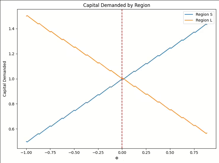
Our first simulation focuses on the net capital positions of regions $S$ and $L$, as determined by the parameter $\Phi \equiv \varepsilon – \theta/4$. Figure 2 illustrates how changes in $\Phi$ affect the capital demanded by each region.

As shown in Figure 2, when $\Phi > 0$, region $L$ becomes a net capital exporter, while region $S$ becomes a net capital importer. This result directly addresses our first research question about how overlapping administrative divisions affect strategic tax-setting behavior. The presence of the overlapping jurisdiction $O$ does not alter the net capital positions of $S$ and $L$ compared to a scenario without $O$.

However, it does influence their tax-setting strategies, as evidenced by the Nash equilibrium tax rates in equation (12). These equations show that $S$ and $L$ adjust their tax rates in response to the overlapping jurisdiction $O$ by factors of $\Gamma(1-\alpha_S)\bar{k}$ and $\Gamma(1-\alpha_L)\bar{k}$, respectively. This strategic adjustment demonstrates how the presence of an overlapping jurisdiction alters tax-setting behavior, even when it doesn’t change net capital positions.

B. Public Good Provision and Welfare Implications

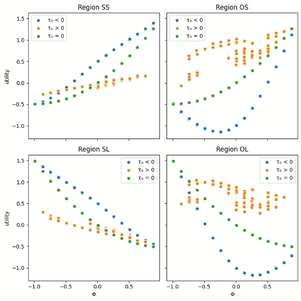
Then, we examine the utility derived from public goods by representative residents in each region. Figure 3 visualizes these utilities across different values of $\Phi$ and $\tau_O$.

Figure 3 reveals several important insights. First, the utility derived from public goods varies significantly across sub-regions ($SS$, $SL$, $OS$, $OL$), highlighting the complex welfare implications of overlapping jurisdictions. Second, the overlapping region $O$’s tax rate ($\tau_O$) has a substantial impact on the utility derived from public goods, especially in the overlapping sub-regions $OS$ and $OL$. Third, the relationship between $\Phi$ and public good utility is non-linear and differs across regions, suggesting that the welfare implications of tax competition are not uniform. These findings suggest that the presence of an overlapping jurisdiction can lead to heterogeneous welfare effects.

C. The Role of the Overlapping Jurisdiction

Our model and simulations highlight the crucial role played by the overlapping jurisdiction $O$. The tax rate of $O$ ($\tau_O^N = \Gamma\bar{k}$) is determined by the proportion of resources allocated from the primary economies ($\alpha_S$ and $\alpha_L$), or specifically $\Gamma$. This relationship reveals that the overlapping jurisdiction’s ability to provide public goods ($H$) is contingent on receiving a sufficient proportion of resources from $S$ and $L$. Specifically, $\alpha_L + \alpha_S$ must exceed $4/3$ for $O$ to provide a positive sum of special public goods.

This finding has important implications for the design of multi-tiered governance systems. It suggests that overlapping jurisdictions need a critical mass of resource allocation to function effectively, which may inform decisions about the creation and empowerment of special-purpose districts or other overlapping administrative structures.

V. Conclusion

This study has examined the dynamics of tax competition in regions with overlapping tax jurisdictions, leveraging game theory to develop a theoretical framework for understanding these administrative structures. By constructing a simplified model and deriving Nash equilibrium conditions, we have identified several key insights that contribute to the existing literature on tax competition. Our analysis reveals that while the introduction of an overlapping jurisdiction does not alter the net capital positions of the primary regions, it leads to strategic adjustments in tax rates. This finding extends the traditional models of tax competition by incorporating the complexities of multi-tiered governance structures.

The effectiveness of the overlapping jurisdiction in providing public goods is found to be contingent on receiving a sufficient allocation of resources from the primary regions. Moreover, our simulations demonstrate that the presence of overlapping jurisdictions can lead to heterogeneous welfare effects across sub-regions, challenging the uniform predictions of traditional tax competition models and suggesting the need for more nuanced policy approaches.

While our study provides valuable insights, it is important to acknowledge its limitations. The use of a simplified model, while allowing for tractable analysis, inevitably omits some real-world complexities. Factors such as population mobility, diverse tax bases, and income disparities among residents were not incorporated into the model. Furthermore, our analysis is static, which may not capture the dynamic nature of tax competition and capital flows over time. The assumption of identical preferences for public goods across all residents may not reflect the heterogeneity of preferences in real-world settings. Additionally, the model assumes perfect information among all players, which may not hold in practice where information asymmetries can influence strategic decisions.

To address these limitations and further advance our understanding of tax competition in a wide array of administrative structures, several avenues for future research are proposed. Developing dynamic models that capture the evolution of tax competition over time, potentially using differential game theory approaches, could provide insights into the long-term implications of overlapping jurisdictions. Incorporating heterogeneous preferences for public goods among residents would allow for a more nuanced examination of how diverse citizen demands affect tax competition and public good provision in overlapping jurisdictions.

Empirical studies using data from regions with overlapping jurisdictions, such as special districts in the United States, could test the predictions of our theoretical model and provide valuable real-world validation. Extending the model to include various policy interventions, such as intergovernmental transfers or tax harmonization efforts, could help evaluate their effectiveness in mitigating potential inefficiencies. Incorporating insights from behavioral economics to account for bounded rationality and other cognitive factors may provide a more realistic representation of tax-setting behavior in complex jurisdictional settings.

In conclusion, this study provides a theoretical foundation for understanding tax competition in regions with overlapping jurisdictions. By highlighting the complex interactions between multiple layers of government, our findings contribute to the broader literature on fiscal federalism and public economics. As urbanization continues and governance structures become increasingly complex, the insights derived from this research can inform policy discussions on decentralization, local governance structures, and intergovernmental fiscal relations. Future work in this area has the potential to significantly enhance our understanding of modern urban governance and contribute to the development of more effective and equitable fiscal policies in multi-tiered administrative structures.

References

[1] C. M. Tiebout, “A pure theory of local expenditures,” Journal of Political Economy, vol. 64, no. 5, pp. 416–424, 1956.
[2] W. E. Oates, Fiscal federalism. Harcourt Brace Jovanovich, 1972.
[3] G. Brennan and J. M. Buchanan, The power to tax: Analytical foundations of a fiscal constitution. Cambridge University Press, 1980.
[4] J. D. Wilson, “A theory of interregional tax competition,” Journal of Urban Economics, vol. 19, no. 3, pp. 296–315, 1986.
[5] G. R. Zodrow and P. Mieszkowski, “Pigou, tiebout, property taxation, and the underprovision of local public goods,” Journal of Urban Economics, vol. 19, no. 3, pp. 356–370, 1986.
[6] D. E. Wildasin, “Nash equilibria in models of fiscal competition,” Journal of Public Economics, vol. 35, no. 2, pp. 229–240, 1988.
[7] R. Kanbur and M. Keen, “Jeux sans fronti`eres: Tax competition and tax coordination when countries differ in size,” American Economic Review, pp. 877–892, 1993.
[8] J. A. DePater and G. M. Myers, “Strategic capital tax competition: A pecuniary externality and a corrective device,” Journal of Urban Economics, vol. 36, no. 1, pp. 66–78, 1994.
[9] O. Hochman, D. Pines, and J.-F. Thisse, “On the optimality of local government: The effects of metropolitan spatial structure,” Journal of Economic Theory, vol. 65, no. 2, pp. 334–363, 1995.
[10] A. Esteller-Mor´e and A. Sol´e-Oll´e, “Vertical income tax externalities and fiscal interdependence: Evidence from the us,” Regional Science and Urban Economics, vol. 31, no. 2-3, pp. 247–272, 2001.
[11] M. Keen and C. Kotsogiannis, “Does federalism lead to excessively high taxes?” American Economic Review, vol. 92, no. 1, pp. 363–370, 2002.
[12] J.-i. Itaya, M. Okamura, and C. Yamaguchi, “Are regional asymmetries detrimental to tax coordination in a repeated game setting?” Journal of Public Economics, vol. 92, no. 12, pp. 2403–2411, 2008.
[13] L. P. Feld, G. Kirchg¨assner, and C. A. Schaltegger, “Decentralized taxation and the size of government: Evidence from swiss state and local governments,” Southern Economic Journal, vol. 77, no. 1, pp. 27–48, 2010.
[14] H. Ogawa and W. Wang, “Asymmetric tax competition and fiscal equalization in a repeated game setting,” International Tax and Public Finance, vol. 23, no. 6, pp. 1035–1064, 2016.

APPENDIX 1 – DERIVING REACTION FUNCTIONS

Let us get the partial derivatives that are needed to get the first order condition of social utility function. Starting with the easier ones,

\begin{align*}
    &\frac{\partial K^*_S}{\partial \tau_S} = -\frac{l}{4}, \quad \frac{\partial K^*_L}{\partial \tau_L} =  -\frac{l}{4}
    , \quad \frac{\partial K^*_O}{\partial \tau_O} = -\frac{l}{3}\left(2-\alpha_L – \alpha_S\right).
\end{align*}

Partial differentiation of $r^*$ with respect to the tax rates are

\begin{align*}
  \frac{\partial r^*}{\partial \tau_S} = -\frac{1}{2}, \quad \frac{\partial r^*}{\partial \tau_L} = -\frac{1}{2}, \quad \frac{\partial r^*}{\partial \tau_O} = -\frac{2- (\alpha_L + \alpha_S)}{2}.
\end{align*}

Then, the partial differentiation of $w^*_i$ with respect to respective tax rates are:

\begin{align*}
    \frac{\partial w^*_S}{\partial \tau_S} &= 2 \left(\frac{K^*_S}{l}\right)\cdot \frac{\partial K_S^*/l}{\partial \tau_S} = -\frac{K^*_S}{2l} \\
    \frac{\partial w^*_L}{\partial \tau_L} &= 2 \left(\frac{K^*_L}{l}\right)\cdot \frac{\partial K_L^*/l}{\partial \tau_L} = -\frac{K^*_L}{2l} \\
    \frac{\partial w^*_O}{\partial \tau_O} &= 3 \left(\frac{K^*_O}{l}\right)\cdot \frac{\partial 3K_O^*/2l}{\partial \tau_O} = -\frac{3(2-\alpha_L – \alpha_S)K_O^*}{2l}.
\end{align*}

Furthermore,

\begin{align*}
     &\frac{\partial K^*_S\tau_S}{\partial \tau_S} = K^*_S -\frac{l}{4}\tau_S, \quad \frac{\partial K^*_L\tau_L}{\partial \tau_L} = K^*_L -\frac{l}{4}\tau_L, \quad \frac{\partial K^*_O\tau_O}{\partial \tau_O} = K^*_O -\frac{l}{3}\left(2-\alpha_L – \alpha_S\right)\tau_O.
\end{align*}

Lastly, we have

\begin{align*}
    \frac{\partial(1-\alpha_S)\tau_O K^*_S}{\partial \tau_S} &= – \frac{l}{4}(1-\alpha_S)\tau_O \\
    \frac{\partial(1-\alpha_L)\tau_O K^*_L}{\partial \tau_L} &= – \frac{l}{4}(1-\alpha_L)\tau_O
\end{align*}

Summing up, the first order condition for the social utility functions of region $S$ and $L$ are:

\begin{align*}
    \frac{\partial U_S}{\partial \tau_S} = l\left(-\frac{K^*_S}{2l} -\frac{\bar{k}_S}{2}\right) + K^*_S -\frac{l}{4}\tau_S – \frac{l}{4}(1-\alpha_S)\tau_O = 0 \\
    \frac{\partial U_L}{\partial \tau_L} = l\left(-\frac{K^*_L}{2l} -\frac{\bar{k}_L}{2}\right) + K^*_L -\frac{l}{4}\tau_L – \frac{l}{4}(1-\alpha_L)\tau_O = 0
\end{align*}

Rearranging the terms, we see that

\begin{align*}
    \tau_S &= -(1-\alpha_S)\tau_O + 2\left(k_S^* -\bar{k}_S\right) \\
    &= -(1-\alpha_S)\tau_O + 2\bigg(\varepsilon + \frac{1}{4}\big((\tau_L – \tau_S – (\alpha_L – \alpha_S)\tau_O ) – (B_L – B_S)\big) \bigg) \\
    &\iff \tau_S^* = \frac{4\varepsilon}{3} – \frac{\theta}{3} + \frac{\tau_L}{3} – \frac{2-3\alpha_S + \alpha_L}{3}\tau_O \\
    \tau_L &= -(1-\alpha_L)\tau_O + 2\left(k_L^* -\bar{k}_L\right) \\
    &= -(1-\alpha_L)\tau_O + 2\bigg(-\varepsilon + \frac{1}{4}\big((\tau_S – \tau_L + (\alpha_L – \alpha_S)\tau_O ) + (B_L – B_S)\big) \bigg) \\
    &\iff \tau_L^* = -\frac{4\varepsilon}{3} + \frac{\theta}{3} + \frac{\tau_S}{3} – \frac{2-3\alpha_L + \alpha_S}{3}\tau_O.
\end{align*}

The FOC for the social utility function of region $O$ is:

\begin{align*}
    &\frac{2l}{3}\left(-\frac{3(2-\alpha_L – \alpha_S)K_O^*}{2l} – \frac{2- (\alpha_L + \alpha_S)}{2}\bar{k}\right) + K^*_O -\frac{l}{3}\left(2-\alpha_L – \alpha_S\right)\tau_O  = 0 \\
    & \iff \tau_O^* = \frac{3(\alpha_L + \alpha_S)-4}{(2-\alpha_L – \alpha_S)(\alpha_L + \alpha_S)}\bar{k} = \Gamma \bar{k}%= \frac{2-3\alpha}{\alpha(2-\alpha)}\bar{k}
\end{align*}

APPENDIX 2 – DERIVING NASH EQUILIBRIUM

Let $\gamma_S$ and $\gamma_L$ be $\Gamma \cdot (2-3\alpha_S + \alpha_L)/3$ and $\Gamma \cdot (2-3\alpha_L + \alpha_S)/3$, respectively. Then,

\begin{align*}
    \tau_S &= \frac{4\varepsilon}{3} – \frac{\theta}{3} + \frac{1}{3}\left(-\frac{4\varepsilon}{3} + \frac{\theta}{3} + \frac{\tau_S}{3} – \gamma_L\bar{k}\right) – \gamma_S\bar{k} \\
    &= \frac{8\varepsilon}{9} – \frac{2\theta}{9} + \frac{1}{9}\tau_S – \left(\frac{\gamma_L}{3} + \gamma_S\right)\bar{k}\\
    &\iff \tau_S^N = \varepsilon – \frac{\theta}{4} – \Gamma\left(1-\alpha_S \right)\bar{k}\\
    \tau_L^N &= -\left(\varepsilon-\frac{\theta}{4}\right) – \Gamma\left(1-\alpha_L\right)\bar{k}\\
    \tau_O^N &= \Gamma\bar{k}
\end{align*}

It follows that

\begin{align*}
    \tau_L^N – \tau_S^N &= -2\left(\varepsilon – \frac{\theta}{4}\right) + \Gamma(\alpha_L – \alpha_S)\bar{k}\\
    \tau_S^N – \tau_L^N &= 2\left(\varepsilon – \frac{\theta}{4}\right) + \Gamma(\alpha_S – \alpha_L)\bar{k}
\end{align*}

Plugging them in, the interest rates and capital demanded in each region are:

\begin{align*}
    r^N &= \frac{1}{2}\left(B_S + B_L\right) – 2\bar{k}\\
    K_S^N &= l\left(\bar{k} – \frac{1}{2}\left(\varepsilon + \frac{\theta}{4} \right)\right) = l\left(\bar{k}_S + \frac{1}{2}\left(\varepsilon – \frac{\theta}{4} \right)\right)\\
    K_L^N &= l\left(\bar{k} + \frac{1}{2}\left(\varepsilon + \frac{\theta}{4} \right)\right) = l\left(\bar{k}_L – \frac{1}{2}\left(\varepsilon – \frac{\theta}{4} \right)\right)\\
    K_{SS}^N &= \frac{2l}{3}\left(\bar{k} + \frac{1}{2}\bar{k}\Gamma(1-\alpha_S) – \frac{1}{2}\left(\varepsilon + \frac{\theta}{4} \right) \right)\\
    K_{SL}^N &= \frac{2l}{3}\left(\bar{k} + \frac{1}{2}\bar{k}\Gamma(1-\alpha_L) + \frac{1}{2}\left(\varepsilon + \frac{\theta}{4} \right) \right)\\
    K_O^N &= \frac{l}{3}\cdot\frac{4 -\alpha_L – \alpha_S}{\alpha_L + \alpha_S}\bar{k}
\end{align*}